An Informal Catalogue of Classic Computer Vision Techniques
“We need to learn how to see a parallel universe composed of activations, keypoints, eigenfaces, feature transforms, classifiers, training sets, and the like.”Trevor Paglen, How to See Like a Machine, Chapter 1
This is a field guide to the ways machines learned to see before deep learning took over in 2012. Each entry shows the technique applied to the same public-domain photograph: a crosswalk in Ginza, Muybridge's galloping horse for motion, a 1941 nightclub for faces. One picture, seen 74 ways. Each entry also names one artwork that uses the technique, where one could be found and checked.
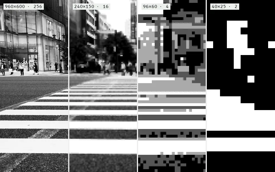
The crosswalk sampled and quantized four ways, left to right (grid · gray levels): a 960×600 grid with 256 gray levels, 240×150 with 16, 96×60 with 4, and 40×25 with only black and white.
A camera or scanner lays a grid over the scene and keeps one number per square, its brightness or color (sampling), rounded to one of a fixed set of steps such as 256 shades of gray (quantization). Every later technique in this catalogue starts from this grid of numbered squares, called pixels. Fewer squares or fewer steps give blockier, flatter pictures.
The machine sees a grid of numbered squares
In the world Every phone sensor, document scanner, satellite and CCTV camera does this first, and the resolution it picks decides whether a face or a license plate is legible to the systems downstream.
In art
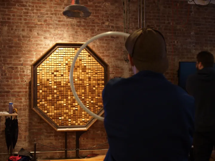
Daniel Rozin, Wooden Mirror (1999). A hidden video camera feeds a computer that reduces the viewer's image to a single gray value for each of 830 square wooden tiles, and a servo motor tilts each tile toward or away from an overhead light to show that value. Rozin's statement calls the reflection 'the least amount of information required to convey a picture (less than an icon on a computer and with no color).' source
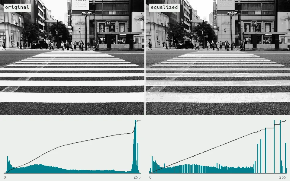
Histogram equalization remaps gray levels so the cumulative curve becomes a straight ramp: the 25% of pixels packed into the top 20 levels (mostly the white stripes) are spread down to level 192, revealing paint texture, and the median moves from 106 to 128.
A histogram is a bar chart that counts how many pixels have each brightness, from black to white. It throws away where things are in the picture and keeps only how much of each tone there is. Equalization uses that count to respread the tones evenly across the whole range, which pulls detail out of murky or washed-out images.
The machine sees a tally of tones with no places in it
In the world Phone cameras read histograms to set exposure, and X-ray, CT, satellite and night-time CCTV software equalizes images to pull detail out of dark or flat areas before a person or an algorithm inspects them.
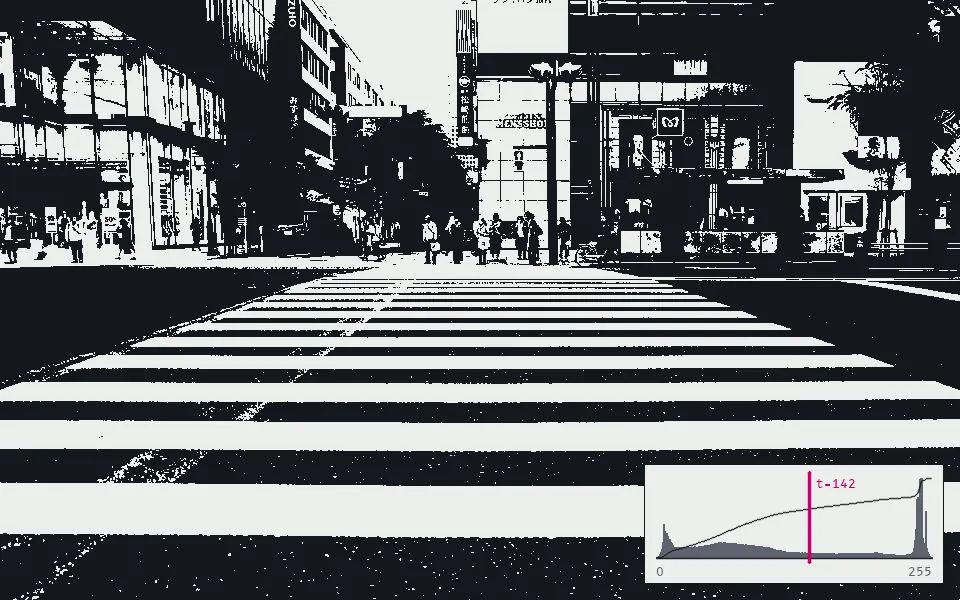
Otsu's method picks gray level 142 as the cut that best separates the histogram's two humps, and the crosswalk becomes ink and paper: 39% of pixels land on the light side.
Thresholding turns a gray picture into pure black and white by picking one cutoff brightness. Every pixel darker than the cutoff goes one way and every lighter pixel goes the other. It is the simplest way to split 'thing' from 'background'. Otsu's method picks the cutoff automatically, choosing the value that best separates the image's dark tones from its light ones.
The machine sees a field of black and white
In the world Document scanners and OCR, barcode and QR readers, factory inspection cameras and license-plate readers binarize images as an early step before they look for shapes or characters.
In art
Camille Utterback and Romy Achituv, Text Rain (1999). Visitors see a mirrored black-and-white video of themselves while colored letters from a poem fall from above. On the artists' page, the letters 'land on anything darker than a certain threshold' and fall again when that dark obstacle moves, so an outstretched arm or a dark coat can catch a word.
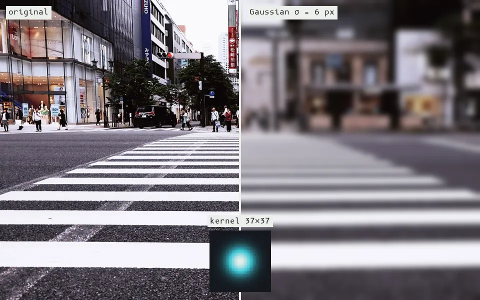
Convolution slides a 37×37 Gaussian kernel (inset, σ = 6 px) across the right half, replacing every pixel with a weighted average of its neighbours, so the stripes and signs soften while large areas of tone survive.
Convolution slides a small grid of weights, called a kernel, across the image and replaces each pixel with a weighted mix of itself and its neighbors. If all the weights are equal, every pixel becomes the average of its patch and the picture blurs. Other weightings sharpen, outline or emboss. Almost every classic vision technique is built from convolutions, and they are also the 'convolution' in the convolutional neural networks of the 2010s.
The machine sees each point as a weighted mix of its neighbors
In the world Camera pipelines denoise and sharpen every photo with convolution kernels; privacy blurring of faces and plates in Street View and bodycam releases is a deliberate blur; and convolutional neural networks run billions of them per image.
In art
Thomas Ruff, nudes (1999-). Ruff downloads pornographic images from the internet, enlarges them, and, per David Zwirner's 2019 release, deliberately manipulates the low-resolution files 'by further blurring the image', turning explicit pictures into soft, painterly ones.
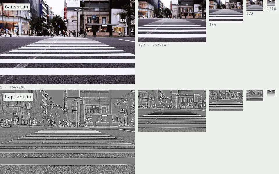
A Gaussian pyramid (top) halves the crosswalk four times, from 464×290 to 29×18, blurring before each step; the Laplacian pyramid (bottom) keeps only what each step threw away, so the stripes' edges live at the fine scales and broad light and dark at the coarse ones.
A pyramid stores the same picture at a ladder of sizes, with each level blurred and shrunk to half the size of the one below, like a stack of smaller and smaller thumbnails. The small, coarse levels hold the big shapes and the large levels hold the fine detail. Searching every level lets a program find a face whether it is near or far, and blending two images level by level makes seams disappear.
The machine sees one scene at every size at once
In the world Face and pedestrian detectors scan image pyramids to catch targets at any distance, and panorama, HDR and portrait-mode blending, image compression and zoomable map tiles all rely on multiscale stacks.
06
Fourier transform
frequency domain · spatial frequency · FFT · discrete cosine transform (DCT)
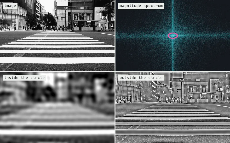
The Fourier transform re-describes the crosswalk as a sum of stripes of every frequency: the bright vertical spine in the spectrum is the crosswalk's horizontal bars, and the 0.5% of frequencies inside the circle carry 62% of the image's contrast energy but rebuild only a blur, while the rest rebuild the edges.
The Fourier transform rewrites a picture as a sum of striped wave patterns of different sizes and angles. Broad, slow waves carry the overall shapes and shading. Tight, fast waves carry edges, texture and fine detail. In this 'frequency' view it is easy to filter out regular noise, blur or sharpen, or compress an image by throwing away detail the eye won't miss.
The machine sees stripes of every size and angle
In the world JPEG and most video codecs use a close relative, the discrete cosine transform, on almost every image online; MRI scanners measure frequency data and transform it into pictures; and satellite and microscopy pipelines filter in the frequency domain.
In art
Thomas Ruff, jpegs (2004-08). Ruff compressed photographs, his own and ones found online, at the JPEG format's maximum rate and then printed them very large, so the grid of pixel blocks left by the compression becomes the picture. source
07
Color spaces and color tracking
HSV · hue thresholding · color segmentation · blob tracking by color
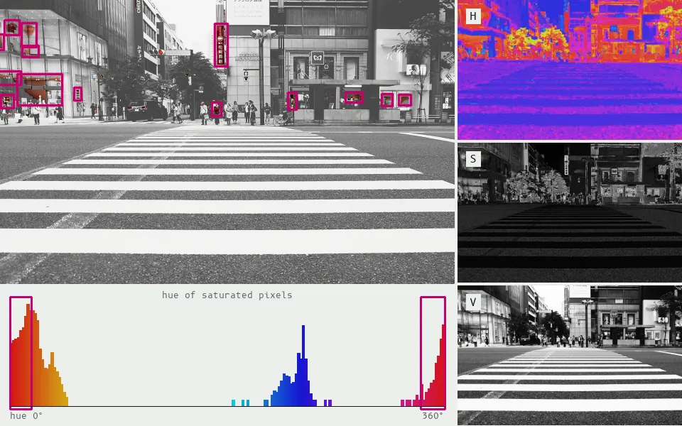
Converted to hue, saturation and value (right), the scene's reds become one band of the hue circle; keeping only pixels with hue between 340° and 16° and saturation above 43% selects 1.1% of the frame, boxed as 14 blobs: signals, a red banner and shop-window displays.
Cameras record color as amounts of red, green and blue, which mixes 'which color' with 'how bright'. Converting to a space like HSV (hue, saturation, value) pulls those apart. A program can then keep only the pixels inside a chosen range, say vivid green, and follow the center of that patch from frame to frame. It is one of the cheapest ways to track something: make it a color nothing else in the scene has.
The machine sees only the pixels of one chosen hue
In the world Optical sorting machines reject discolored grain, fruit and recycled plastic by color; robots follow colored markers; and the PlayStation Move controller's glowing ball is located by its color.
In art
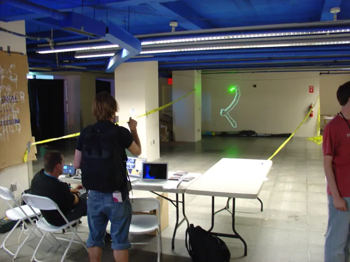
Graffiti Research Lab (Evan Roth, James Powderly, Theo Watson), L.A.S.E.R. Tag (2007). A camera watches a building while someone writes on it with a green laser pointer. Watson's open-source software picks out the dot by color, using settings for a hue point, a hue range, a minimum saturation and a minimum brightness, and a high-power projector paints the tracked strokes back onto the facade at architectural scale. source
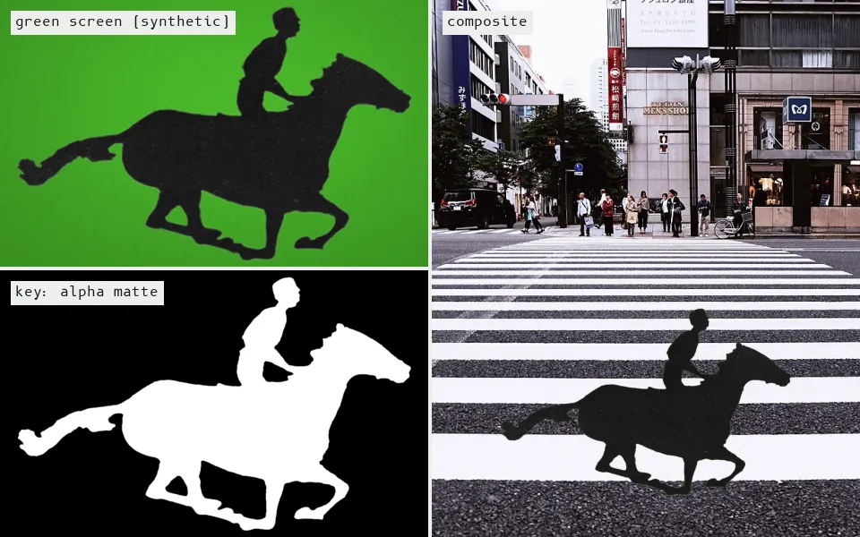
Chroma keying measures each pixel's distance from the backdrop's green in the colour (CbCr) plane and turns it into transparency: here 75% of a synthetic green-screen shot of Muybridge's horse keys out, and the rest is laid over the crosswalk.
Chroma keying makes one chosen color transparent. A subject is filmed in front of an evenly lit blue or green backdrop, and every pixel close to that color is replaced by the matching pixel from another picture. The weather presenter standing in front of a moving map is the familiar example. Done photochemically in film from 1940, it became an electronic, real-time effect in television.
The machine sees one color as a hole to see through
In the world TV news and weather, film and virtual-production stages, livestream setups and video-conference backgrounds all key out a color (or, now, a learned matte) to composite people into other scenes.
In art
Peter Campus, Three Transitions (1973). Made at Boston's public-TV station WGBH, the video uses chroma key on Campus's own body. In the second transition he paints his face with blue key color, and the paint becomes a window onto another image of his face; in the third he burns a keyed image of his face like a photograph. source
09
Image averaging and composites
composite portrait · mean image · amalgamation · frame averaging
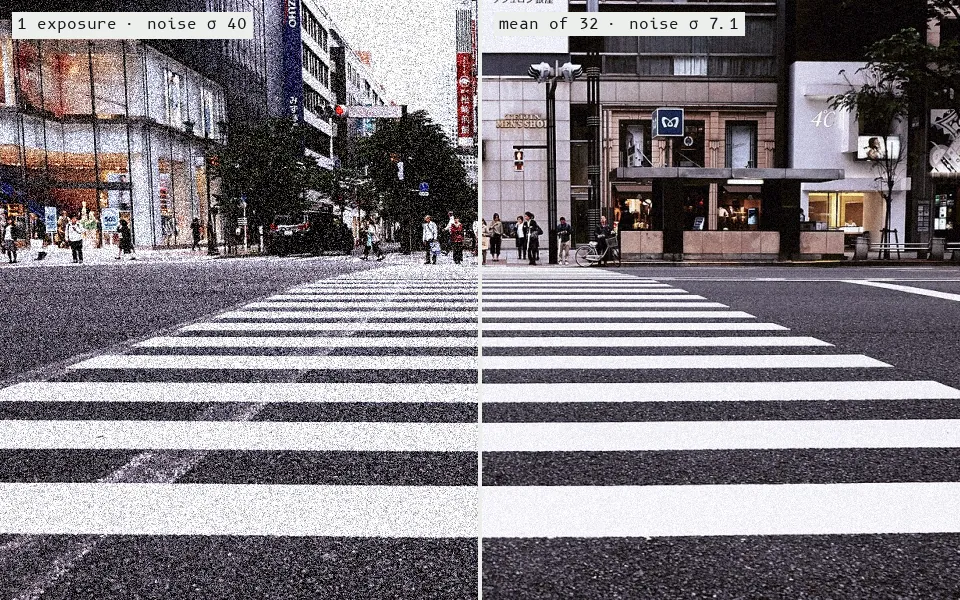
Averaging 32 exposures that each carry random sensor noise (left, σ = 40 gray levels; the noise is simulated) cancels the noise and keeps the scene (right, σ = 7.1), close to the 1/√32 that statistics predicts.
Averaging lines up many images and, at every pixel, takes the mean of their values. Whatever the images share comes through clearly, and whatever differs fades into a soft blur. Francis Galton did this with faint successive exposures on one photographic plate, hoping to reveal human 'types', including supposed criminal types. Computers made it a one-line operation.
The machine sees the blur of what many faces share
In the world Stacking many frames cuts noise in astronomy, microscopy and phones' night modes, and face recognition subtracts an average 'mean face' before computing eigenfaces.
In art
Jason Salavon, The Class of 1988 & The Class of 1967 (1998). In the artist's words, the works 'apply a custom averaging process to graduating yearbook photos from my family history': every senior portrait from his 1988 high-school class, and from his mother's 1967 class in the same hometown (Fort Worth, Texas), merges into one hazy composite. Salavon wrote the averaging code himself in C on SGI workstations.
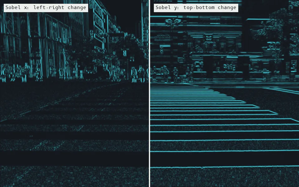
Sobel filters measure how fast brightness changes in each direction: the horizontal filter (left) sees the building edges and poles but is nearly blind to the stripes, which the vertical filter (right) picks up; on the road it responds 3.7 times more strongly.
An image gradient measures, at every pixel, how fast the brightness is changing and in which direction. The Sobel and Prewitt operators do it with a tiny 3 x 3 grid of weights that compares the pixels on one side of a point with those on the other. Flat areas come out black, and boundaries where light meets dark come out bright, so the result looks like a glowing outline drawing.
The machine sees only where light turns to dark
In the world Gradients are the first step in most edge and feature detectors (Canny, SIFT, HOG pedestrian detection); camera autofocus maximizes gradient strength; and inspection systems use them to locate and measure part edges.
In art
Rafael Lozano-Hemmer, Body Movies, Relational Architecture No. 6 (2001). Thousands of portraits are projected onto a building facade, washed out by floodlights except inside the shadows of passers-by. A camera watches the facade, and custom software finds the edges of those shadows to decide when they have uncovered every portrait. source
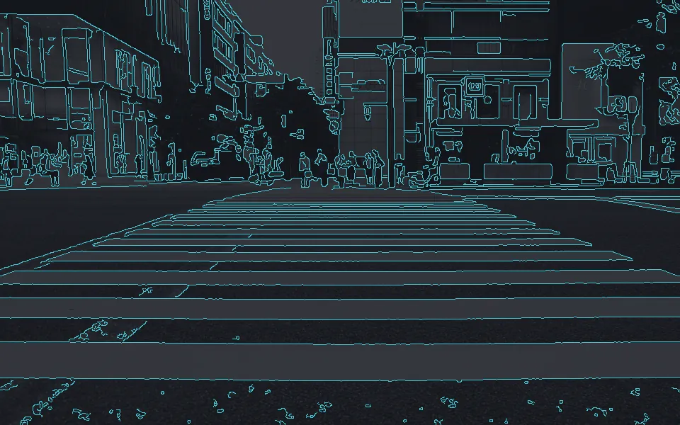
Canny's detector smooths the image, finds the gradient, thins it to one-pixel ridges and keeps ridges stronger than 140 or connected to one stronger than 50: 7.6% of the crosswalk's pixels survive as edges.
Canny's method turns a photo into a clean drawing of thin edge lines. It first blurs the image slightly to calm the noise, then measures brightness gradients. Next it thins each edge to a one-pixel ridge, and finally it keeps weak edge pixels only where they connect to strong ones. Canny derived it from three goals: find the real edges, place them accurately, and mark each edge only once.
The machine sees a thin-line drawing of every boundary
In the world It is the default edge detector in OpenCV and most vision libraries, used for lane detection in driver-assistance systems, for finding document and card edges in phone scanner apps, and before Hough line and circle detection.
12
Hough transform
line detection · Hough circle transform · voting · accumulator
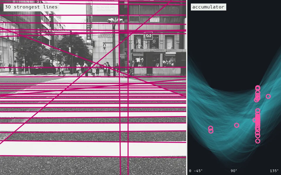
The Hough transform lets every edge pixel vote for all the lines that could pass through it; votes pile up in the (θ, ρ) accumulator (right), and its 30 strongest peaks become the lines drawn on the scene, 26 of them near-horizontal: stripe edges, building ledges and signs.
The Hough transform finds straight lines, and in later versions circles, even when they are broken or noisy. Every edge pixel 'votes' for all the lines that could pass through it. The votes pile up in a tally table, and the lines with the most votes win. It was invented to trace the paths of subatomic particles in bubble-chamber photographs.
The machine sees the lines and circles that collect the most votes
In the world Lane-departure warning systems, document deskewing, reading dials and gauges, locating round parts on assembly lines, and finding irises, coins and pupils all use Hough voting.
In art
Trevor Paglen, Shoshone Falls Hough Transform; Haar (2017). Paglen photographed Shoshone Falls, which Timothy O'Sullivan photographed in 1874 for the Wheeler Survey's 'reconnaissance' of the American West, and overlaid the strokes and lines two computer-vision algorithms 'see' in it. The Smithsonian says one of them 'surveyed the image for underlying lines, a technique used in self-driving cars and robotics.'
13
Contour tracing
border following · findContours · chain code · outline extraction
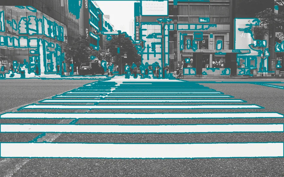
Border following (Suzuki and Abe's algorithm) walks the edge of every white region in the thresholded crosswalk and records it as a chain of pixels: 131 closed contours, the longest on the road traced by 4,017 boundary points.
Contour tracing walks around the edge of each white shape in a black-and-white image, pixel by pixel, and records its outline as a list of points. That turns a blob of pixels into a shape a program can measure, draw or compare. Suzuki and Abe's version also tells outer boundaries apart from the holes inside them, building a family tree of shapes within shapes.
The machine sees outlines, and the holes inside them
In the world Factory inspection uses it to find and measure parts, microscopy to count cells and nuclei, OCR to separate characters, and camera interfaces to follow hand and body silhouettes.
In art
Golan Levin, Interstitial Fragment Processor (2007). Visitors cast shadows on a wall, and the software 'recovers, collects and drops the contours formed as enclosed holes in the shadows of its participants'. The gap made by a hand on a hip, for example, becomes a soft object that falls to the floor and makes a sound.
14
Polygon approximation
Ramer-Douglas-Peucker · line simplification · approxPolyDP · corner finding
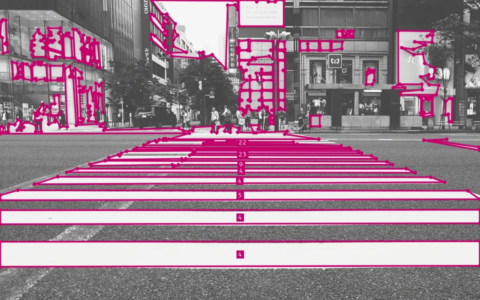
Douglas–Peucker simplification replaces each traced outline with the fewest straight segments that stay close to it: the 5 nearest stripes, 8,978 boundary pixels in all, become polygons of 4–5 vertices (labelled), while the far stripes, which run together with the lane marking, need up to 23.
Polygon approximation simplifies a wiggly outline into a few straight segments. The Ramer-Douglas-Peucker method draws a line between the two ends, finds the point that strays farthest from it, and, if that point strays more than a set tolerance, keeps it as a corner and repeats on each half. A wobbly hand-drawn square becomes four corners, and a coastline becomes a handful of points.
The machine sees a shape as a few corners
In the world It simplifies coastlines, roads and GPS tracks for digital maps, and finds the four corners of documents, screens, AR markers and license plates before they are flattened and read.
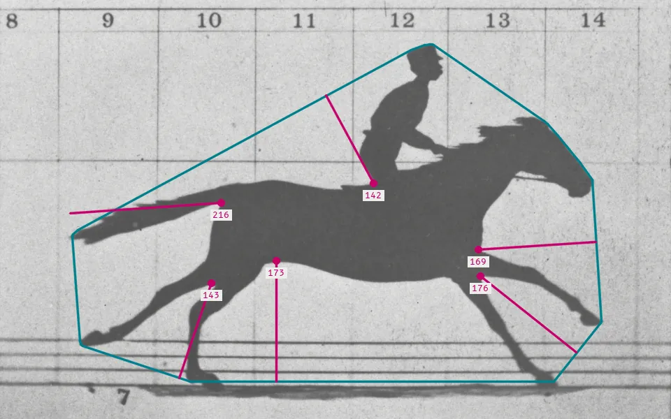
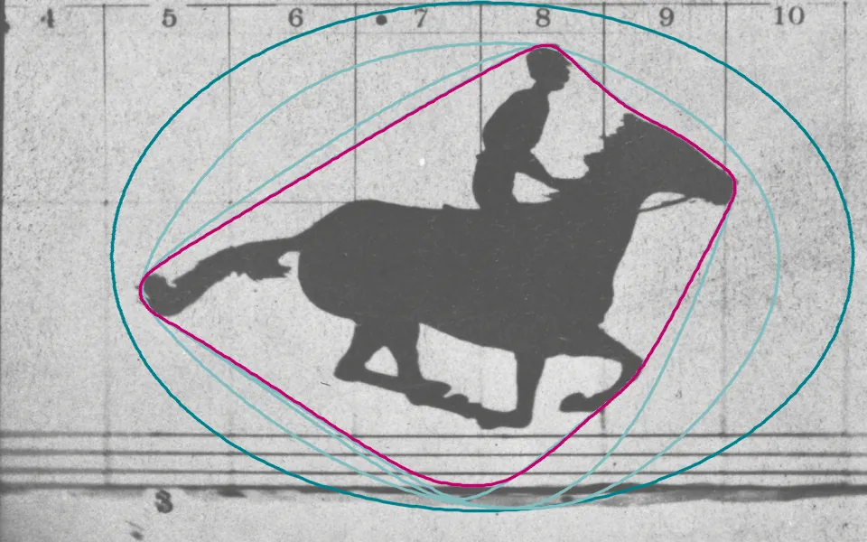
The convex hull (cyan) is the tightest rubber band around the horse; the gaps between it and the silhouette are convexity defects, the six deepest marked with their depth in pixels, and the horse fills 38% of its hull.
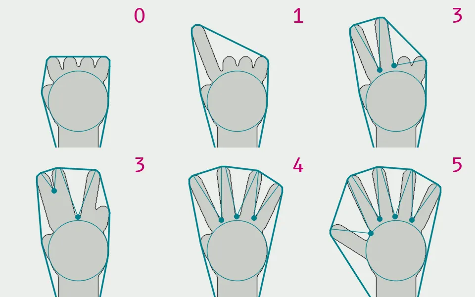
The convex hull is the shape you get by snapping a rubber band around an outline: it touches the outermost points and skips every dent. Comparing the hull with the real outline exposes the 'convexity defects', the pockets between them, such as the gaps between spread fingers. Counting the deep pockets is a classic way to count raised fingers.
The machine sees a rubber band around a shape, and the gaps inside it
In the world Camera-based hand-gesture interfaces count fingers from convexity defects, robots use hulls for collision checks and grasp planning, and inspection systems use them to spot chips and breaks in parts and pills.
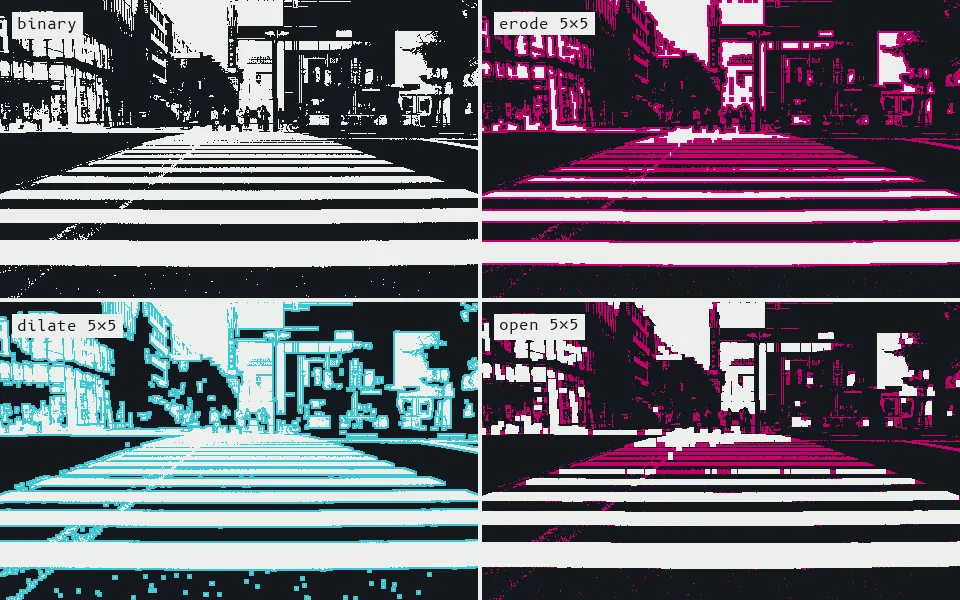
Morphology probes a binary image with a small square: erosion strips 51% of the white (magenta), dilation grows it (cyan), and opening, an erosion then a dilation, wipes out specks too small to hold the square, cutting the white regions from 501 to 72.
Morphological operations reshape black-and-white shapes using a small stamp called a structuring element. Erosion shaves pixels off every edge and dilation adds them. Erosion followed by dilation ('opening') wipes out specks of noise, and dilation followed by erosion ('closing') fills small holes and gaps. The method began as a way to measure grains in slices of rock.
The machine sees shapes that can be shaved down and swollen up
In the world Nearly every segmentation pipeline uses it to clean up masks: circuit-board and semiconductor-wafer defect inspection, cell counting in microscopy, fingerprint cleanup, and removing specks before license-plate characters are cut apart.
17
Distance transform
distance map · chamfer distance · grassfire transform · signed distance field
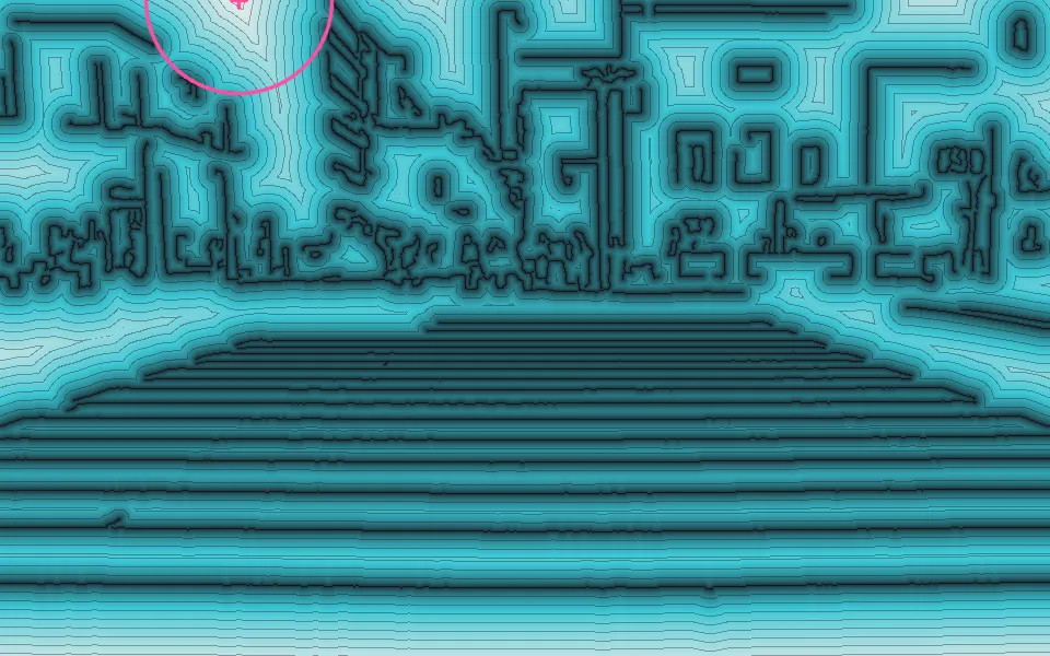
The distance transform gives every pixel its distance to the nearest Canny edge (black), drawn here with a contour every 8 px; the emptiest spot is 85 px from any edge, the circle in the sky.
A distance transform takes a black-and-white shape and replaces every pixel with its distance to the nearest edge. The middle of a thick region becomes bright and the rim stays dark, which turns the shape into a smooth hill. The hill's ridge traces the shape's center line, and any value says how far that point is from an obstacle.
The machine sees every point labeled by how far it is from an edge
In the world Robots and drones use distance maps to plan paths that stay clear of obstacles; they also drive chamfer matching of outlines and the separation of touching cells or coins before watershed segmentation; and games and interfaces render sharp text from signed distance fields.
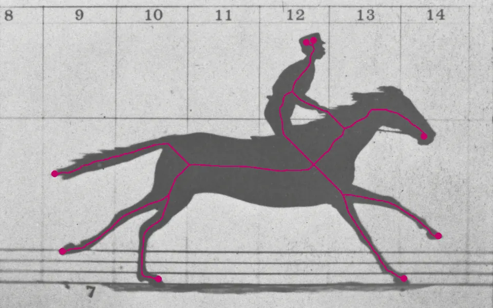
Thinning erodes the silhouette from every side until only a one-pixel-wide medial line is left, a stick figure that keeps the horse's topology: 8 limbs and extremities end in the dots, after spurs under 40 px are pruned.
Skeletonization shrinks a shape to a one-pixel-wide center line that keeps its branches, the way a stick figure keeps a body's pose. Harry Blum pictured lighting a fire along the shape's whole edge at once: the lines where the flame fronts meet form the 'medial axis'. Thinning algorithms reach the same result by peeling away edge pixels layer by layer without ever breaking the shape apart.
The machine sees a stick figure of every shape
In the world Fingerprint systems thin ridges to find minutiae (ridge endings and splits), and the technique also serves OCR and handwriting recognition and the mapping of roads, rivers and blood vessels in aerial and medical images.
In art
Golan Levin, Ghost Pole Propagator II (2016). The installation uses 'skeletonization (or the medial axis transform)' to compute stick figures in real time from the silhouettes of visitors and passers-by. A computer-controlled laser then draws the moving skeletons at huge scale, alongside the recorded stick figures of earlier participants.
An active contour starts as an ellipse (dashed) and shrinks under its own tension until image edges hold it; snapshots after 100, 300 and 1,000 steps (pale) lead to the outline after 3,000 (magenta), which settles on the rider, nose, hooves and tail but, kept smooth by its stiffness, never reaches into the gaps between the legs.
A snake is a stretchy, springy loop that a program drops near an object and lets settle. Its 'energy' rewards lying on strong edges and penalizes bending and stretching, so it slithers into a smooth outline that hugs the object's boundary. Restarted from its last position in each new frame, it can follow a moving or changing shape.
The machine sees an elastic loop tightening onto an outline
In the world Medical imaging tools use active contours to outline organs, tumors and heart chambers in MRI, CT and ultrasound, and they also appear in lip and face-contour tracking and in rotoscoping tools for film.
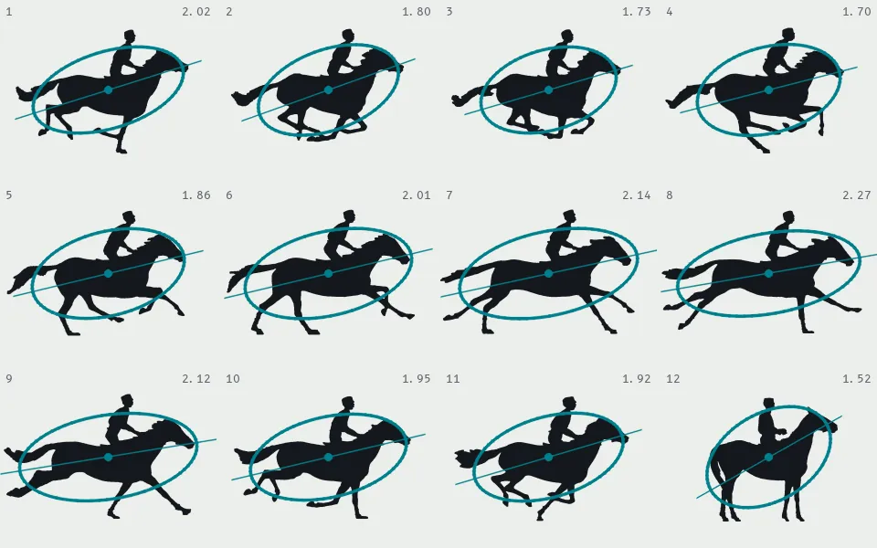
Image moments boil each silhouette down to a few numbers: the centroid (dot), the principal axis and the ellipse with the same spread; elongation (top right) runs 1.70–2.27 through the gallop, and by Hu's moment invariants frame 12, the standing horse, is the odd one out.
Shape descriptors boil a shape down to a few numbers. 'Moments' are weighted sums over a shape's pixels that give its area, center of mass and tilt. Hu combined them into seven numbers that stay the same when the shape is moved, resized or rotated. Two shapes with similar numbers are treated as the same kind of thing.
The machine sees a shape reduced to a short list of numbers
In the world They sort and orient parts on conveyor belts, classify cells and particles in microscopy, and recognize characters and hand poses; early gesture systems matched silhouettes this way.
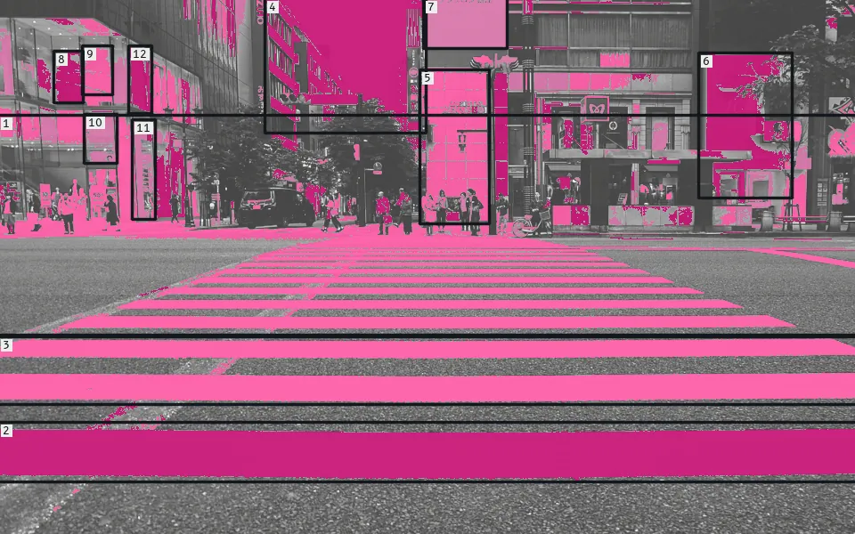
Connected-component labelling gives every white region of the thresholded crosswalk its own number by flooding outward through touching pixels: 1895 regions, 226 of them at least 20 px, the 12 largest boxed and ranked by area.
Once an image has been split into figure and ground (say, white body pixels on black), connected-components labelling walks the grid and gives every group of touching figure pixels its own number. Each numbered group becomes a 'blob' that can be counted and measured by its area, centre and bounding box, and followed from frame to frame. From this step on, the machine is working with things it can count, not loose pixels.
The machine sees countable islands of pixels
In the world People and vehicle counters, the step in license-plate readers that isolates each character, and part inspection on factory lines all begin by labelling blobs.
In art
Scott Snibbe, Boundary Functions (1998). An overhead camera watches people walking on a gallery floor, and software picks each one out of the video as a separate figure. It then projects lines between them, dividing the floor into the region closest to each person, a Voronoi diagram.
22
Region growing and flood fill
paint bucket · seed fill · region growing · magic wand
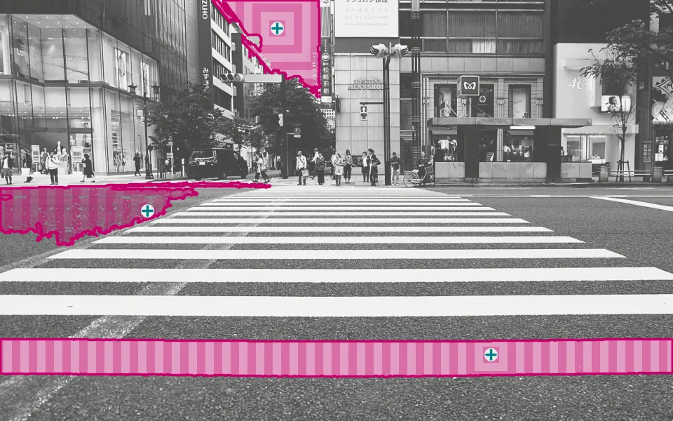
Region growing starts at a seed (cross) and keeps absorbing neighbours whose colour is within a few levels of the pixel they grew from; bands mark every 12 steps of the spread, and the three seeds claim 2.0% (sky), 8.4% (one stripe) and 2.5% (asphalt beside the crossing) of the frame.
Start at one seed pixel and keep absorbing neighbouring pixels that look similar enough, whether the same colour or within a tolerance, until the similarity runs out. Flood fill is the paint-bucket tool. Region growing is the same idea used to carve an image into areas. The boundary of the result is simply wherever the similarity stopped.
The machine sees everything connected to here that looks like here
In the world The paint-bucket and magic-wand tools in image editors, and region growing in medical imaging, where a clicked seed point grows into the outline of an organ or lesion.
In art
Jürg Lehni, Flood Fill (2003–). Lehni deliberately slows the paint-bucket algorithm down so you can watch it work, with pixels flowing into their shapes 'like sand into a container'. In animations such as Flood Fill – Clock and Flood Fill – Verbs (both 2009), the fill's step-by-step spread from a seed point is the whole subject.
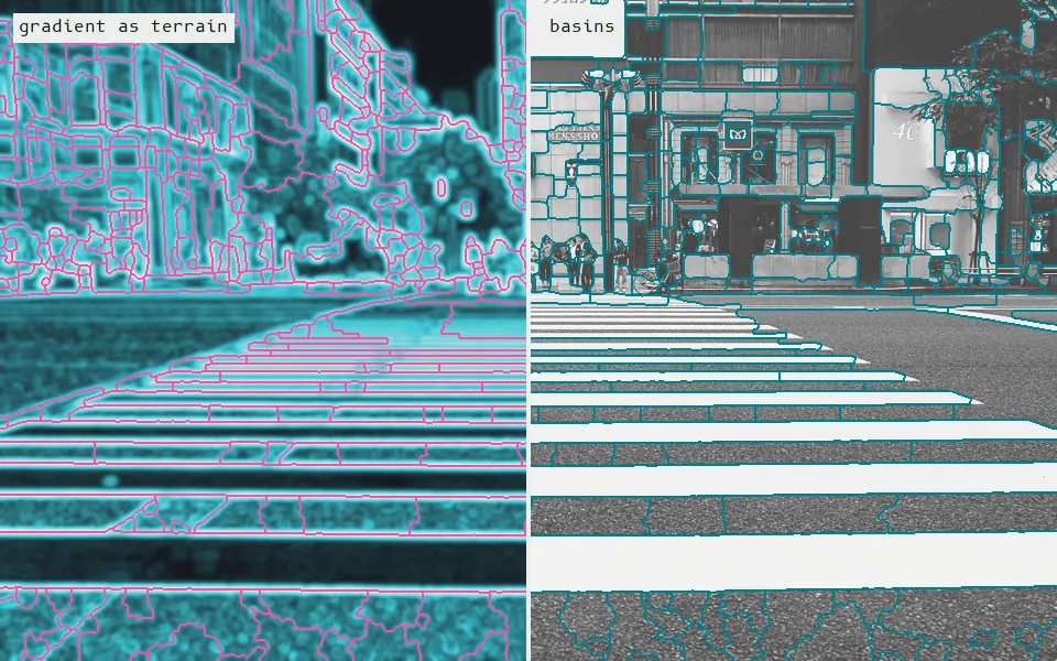
Watershed treats the gradient image as terrain (left, bright = steep) and floods it from its 584 deepest hollows; where two floods meet it builds a dam, and the dams (right) cut the crosswalk into 584 basins.
Treat the image's brightness, or its edge strength, as a landscape where bright is high ground and dark is valley. Flood it from the lowest points, and wherever water from two different basins would meet, build a dam. The dams become the boundaries and each basin becomes a region. Run as is, it splits the image into far too many pieces, so it is usually started from chosen 'marker' seeds.
The machine sees a terrain of basins and ridgelines
In the world Separating touching cells and nuclei in microscope images, grains in materials science, and touching objects in industrial inspection.
In art
Trevor Paglen, CLOUD #603 Watershed (2019). A photograph of a cloud, overlaid with the marks a watershed algorithm leaves when it divides the sky into basins. It belongs to Paglen's CLOUDS series, which shows the sky as computer-vision algorithms carve it up, and the title names the algorithm. It was shown in Paglen's The Shape of Clouds at Pace, Geneva.
24
k-means color clustering
color quantization · dominant-color extraction · Lloyd's algorithm
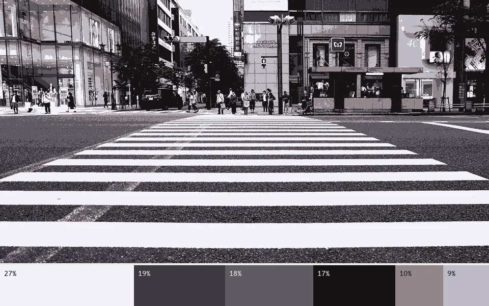
k-means sorts every pixel into the nearest of 6 colours and moves each colour to the average of its pixels until nothing changes; the crosswalk comes back painted with six inks, in the proportions shown below (largest 27%, smallest 9%).
Choose a number k, say five. Treat each pixel's colour as a point in colour space and drop k guesses for 'typical colours' among the points. Assign every pixel to its nearest guess, move each guess to the average of its pixels, and repeat until nothing changes. The image collapses to k colours, a palette the machine has decided best sums it up.
The machine sees five colours, and which pixels belong to each
In the world Colour reduction for GIFs and limited palettes, the 'dominant colours' that design and shopping tools pull from images, and a first step in many segmentation pipelines.
In art
Frederic Brodbeck, Cinemetrics (2011). Brodbeck's graduation project at the Royal Academy of Art in The Hague splits a film into shots and draws the whole film as a ring-shaped 'fingerprint'. For colour, his own script clusters each shot's pixels into five colours with k-means (scipy's kmeans2, NUM_CLUSTERS = 5) and uses them as that shot's palette. source
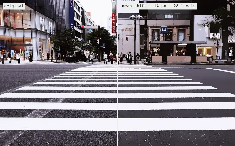
Mean-shift filtering moves every pixel uphill to the densest nearby cluster of similar colours (within 14 px and 28 levels), so each region settles on one shared colour: on the right the number of distinct colours falls from 6,806 to 2,424 while edges stay sharp.
Describe every pixel by its colour and its position. Each pixel then repeatedly moves toward the densest crowd of similar pixels nearby, climbing a density map until it settles on a peak. Pixels that end on the same peak form one segment. Unlike k-means, you don't choose how many regions you get; you choose how wide 'nearby' is.
The machine sees pixels drifting toward their densest neighbours
In the world Edge-preserving smoothing and segmentation in photo-editing and remote-sensing software, and, as CamShift, colour-based object tracking.
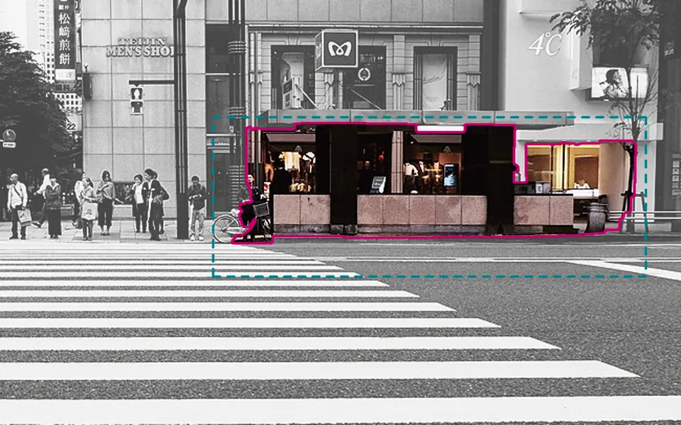
GrabCut is given only a rough box (dashed) around the low pavilion on the far corner, in a detail of the scene; it models the colours inside and outside as two mixtures and repeatedly cuts the pixel graph where they disagree most, keeping 59% of the box as foreground (magenta outline).
You drag a rough box around the thing you want. The algorithm learns a colour model for 'inside' and one for 'outside', then treats the image as a network in which neighbouring pixels are tied together and each pixel is pulled toward foreground or background. Cutting the network where it is cheapest to cut separates the object from its background. It then refits the colour models and cuts again until the outline settles.
The machine sees the cheapest line between figure and ground
In the world One-click background removal in photo and office software, product cut-outs for online shops, and annotation tools for labelling training data.
27
Superpixels (SLIC)
SLIC · simple linear iterative clustering · oversegmentation
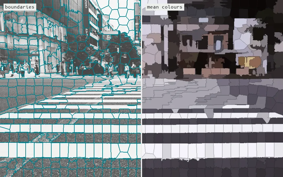
SLIC clusters pixels by colour and position at once, growing 566 compact superpixels that hug the edges (left); filled with their average colour (right), they reduce the 576,000-pixel frame to 566 regions while keeping its outlines.
SLIC scatters seed points in a grid over the image and grows a compact patch around each one by gathering nearby pixels of similar colour. In effect it is k-means confined to small neighbourhoods. The image becomes a few hundred tile-like patches that follow its edges, so later steps can reason about hundreds of patches instead of millions of pixels.
The machine sees a mosaic of colour-coherent tiles
In the world Speeding up segmentation in medical and satellite imaging, and the patches that explanation tools such as LIME switch on and off to show which parts of an image a classifier relied on.
28
Saliency maps
visual saliency · bottom-up attention model · Itti–Koch model
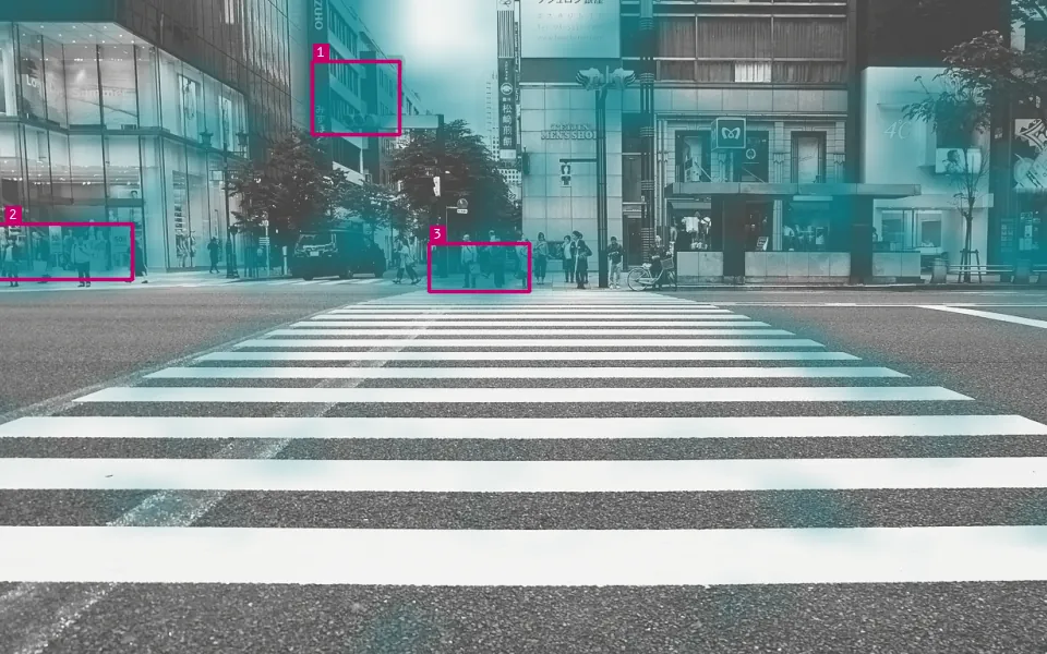
Spectral-residual saliency (Hou and Zhang, 2007) strips out what is statistically typical of natural images and keeps the surprises: 2% of the crosswalk scores more than three times the average, and the three strongest regions are boxed and ranked.
A saliency map is a guess at where a person's eyes will land first. Itti and Koch's model measures, at several scales, how much each spot differs from its surroundings in brightness, colour and edge direction. It adds these 'pop-out' maps into one heat map, and the brightest spots are predicted to catch attention first.
The machine sees what sticks out
In the world Automatic thumbnail cropping, video compression that spends detail where viewers look, testing ad and packaging layouts, and steering where robots and cameras look.
No single inventor; Ramesh Jain & Hans-Hellmut Nagel's 'difference pictures' are a standard early citation, 1979, On the Analysis of Accumulative Difference Pictures from Image Sequences of Real World Scenes (IEEE PAMI)
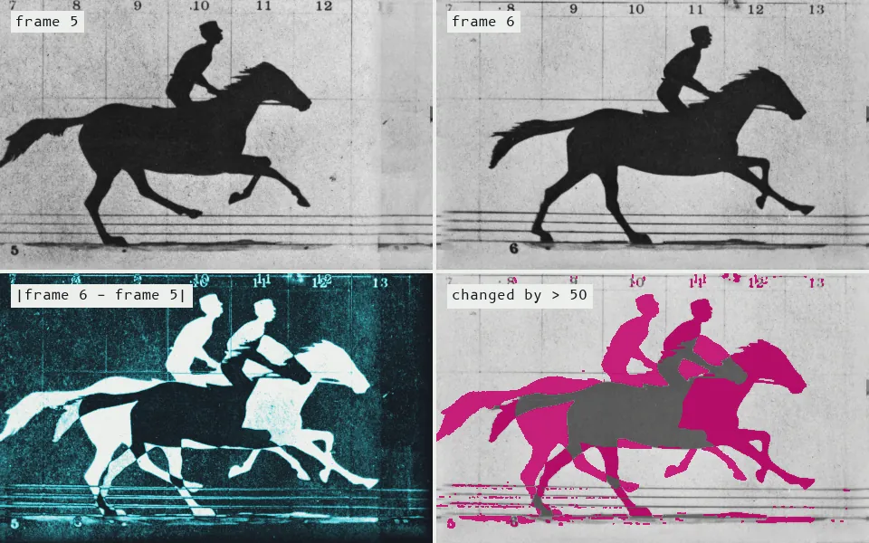
Subtracting one exposure from the next leaves only what changed: 19.7% of the view differs by more than 50 gray levels, a double horse that marks both where it was and where it is, while the part of the dark body that overlaps itself between frames cancels out.
Subtract each video frame from the one before it, pixel by pixel. Where nothing moved, the difference is close to zero; where something moved, it lights up. Apply a threshold and you have a cheap, fast motion detector that knows nothing about what moved, only that something did.
The machine sees only what changed since a moment ago
In the world Motion-triggered recording in security cameras and video doorbells, video compression (which mostly stores the differences between frames), and early camera-based games and installations.
In art
David Rokeby, Very Nervous System (1986–1990). Video cameras watch a space, and a computer turns visitors' movements into sound and music in real time. As MIT Technology Review described it, the computer 'extracts motion from a video signal by comparing one frame with the last and determining which pixels have changed.' source
30
Background subtraction
foreground detection · background modelling · Gaussian mixture background model
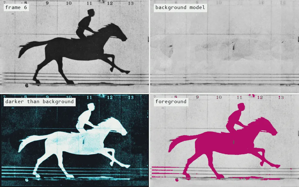
Background subtraction compares each frame with a model of the empty scene, here each pixel's 85th-percentile brightness across all eleven registered plates; whatever is more than 50 gray levels darker is foreground, 19% of the view, 93% of it in one blob: horse, rider and shadow.
Keep a picture of the scene with nobody in it and compare each new frame against it: whatever differs is 'foreground'. Real scenes change, with clouds, swaying trees and lights switching on, so Stauffer and Grimson model each pixel as a small mix of its usual colours and keep updating the mix. A pixel counts as foreground only when it fits none of them. Unlike frame differencing, a person who stops moving stays visible.
The machine sees whatever isn't usually there
In the world Traffic counting, people counting in shops and stations, CCTV analytics that flag loitering or unattended bags, and graphics drawn onto sports broadcasts.
In art
David Rokeby, Sorting Daemon (2003). A robotic camera pans the street outside the Goethe-Institut Toronto looking for moving things that might be people. When it finds one, in Rokeby's words, 'it removes the person's image from the background'. It then breaks the cut-out figure into patches of similar colour and sorts them by hue into a large projected composite. Rokeby made it in response to automated profiling in the 'war on terrorism'.
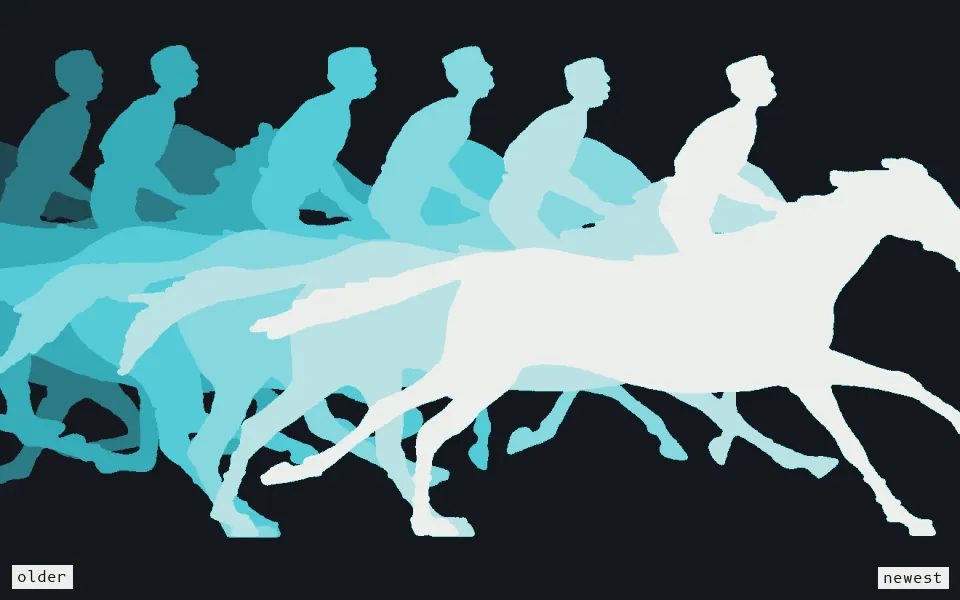
A motion-history image stamps each new silhouette over the fading older ones, so 7 exposures, about a quarter of a second, collapse into one picture that runs from dim (old) to bright (newest): where the motion came from and where it is now.
Stack a moving silhouette over time into a single image where the newest motion is brightest and older motion fades toward black. One still frame then shows where something moved and in which direction, from dim to bright. Bobick and Davis used these 'temporal templates' to recognise actions such as sitting down or raising the arms.
The machine sees a gesture as a fading smear
In the world Early gesture and action recognition, simple camera interfaces for games and kiosks, and activity detection in surveillance research; OpenCV's early 'motion templates' functions implement it.
In art
Ed Tannenbaum, Recollections (early 1980s). A camera captures the visitor's silhouette, colours it according to the moment it was recorded, and adds it to a large projection. Movement builds up into rainbow trails of past and present bodies. It is the same idea as a motion history image, silhouettes marked by time and accumulated, made about fifteen years before Bobick and Davis named it. source
32
Optical flow
dense motion field · Horn–Schunck · motion vectors
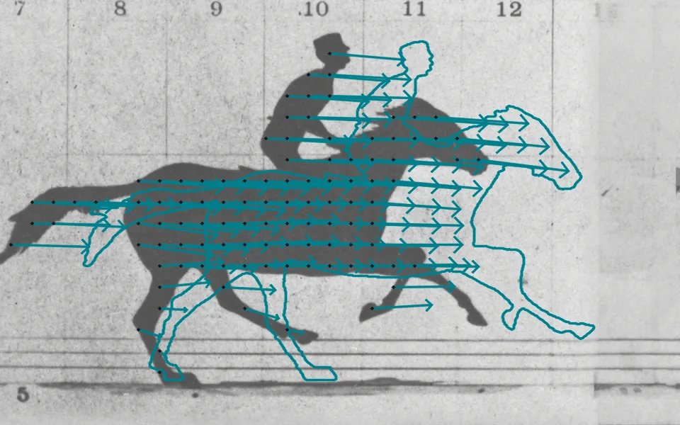
Dense optical flow (DIS) estimates, for every pixel of frame 5, where it went in frame 6; drawn from the horse's pixels, the arrows land on frame 6's outline (cyan), a median shift of 156 px, about 22 inches of track in 1/25 s; on the plain backdrop the motion is undetermined, so no arrows are drawn there.
For every point in a frame, estimate which way it moved, and how far, by the next frame, so the picture becomes a field of tiny arrows. Horn and Schunck assumed that a point keeps its brightness as it moves and that neighbouring points move alike, then solved for the smoothest arrow field consistent with both. Unlike frame differencing, flow gives direction and speed, not just 'something changed'.
The machine sees a field of arrows
In the world Video stabilisation in phones, slow-motion frame interpolation, navigation for drones and robots, and motion analysis of sports and traffic footage.
In art
Frieder Weiss, Flow (None). An interactive floor projection at the phaeno science centre. An infrared camera above the floor records visitors' movements, and according to the exhibit text the projected currents are 'calculated by means of the mathematical model of the optical flow'. Walking stirs the floor like churning water, and spinning with outstretched arms makes a vortex. source
33
Feature tracking (KLT)
Kanade–Lucas–Tomasi tracker · Lucas–Kanade · good features to track · point tracking
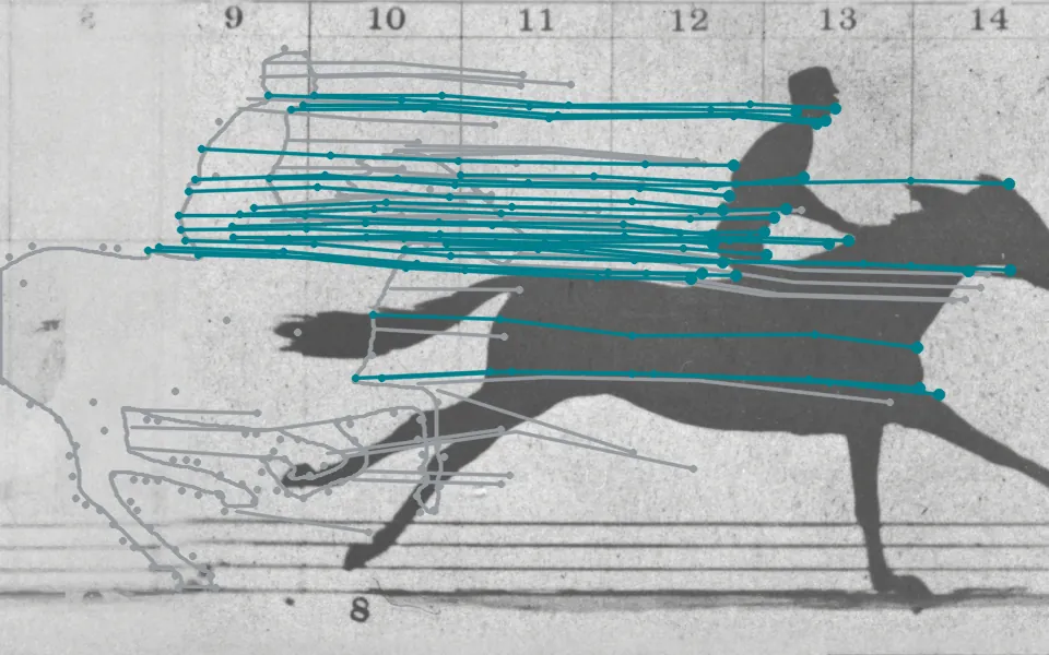
The Kanade–Lucas–Tomasi tracker picks 159 corners on the horse in frame 4 and follows each small patch from exposure to exposure (frame 4's outline in gray); 26 survive to frame 8 (cyan), mostly on the rider and the head, moving a median 167 px per frame, while patches on the legs, whose shape changes between exposures, are lost (gray).
Pick small patches that are easy to follow, usually corners where the texture changes in two directions (Shi and Tomasi's 'good features to track'). For each patch, look in the next frame for where it went by nudging the patch's position until it matches best. The result is a few hundred points, each with a trail, which is enough to estimate how the camera or the objects moved.
The machine sees a constellation of trackable corners
In the world Video stabilisation, match-moving in visual effects, early face tracking in phone apps, and visual odometry for drones and robots.
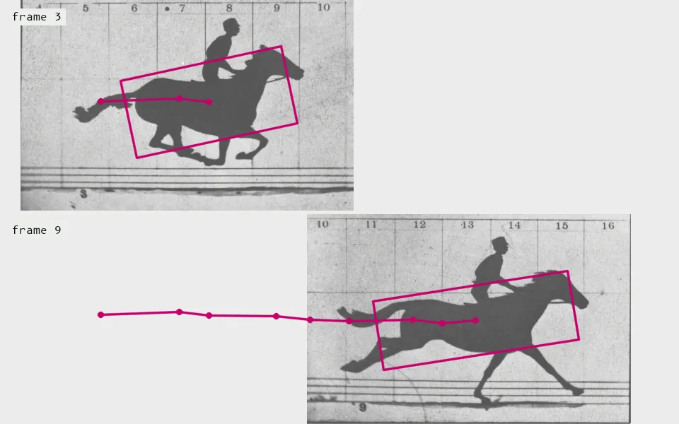
CamShift turns each frame into a map of how horse-like every pixel's gray level is, then climbs that map with a window that re-sizes and turns itself to fit; started on frame 1's silhouette it follows the horse the length of the run, ending as a 783×276 px box (path of window centres in magenta).
Build a histogram of the target's colours, say a face's skin tones, then turn each new frame into a map of how likely each pixel is to be that colour. Mean shift slides a window uphill to the densest part of that map, and CamShift also resizes and tilts the window as the target comes closer, moves away or turns. It is fast and needs no training, but anything else of the same colour can fool it.
The machine sees a blob of the right colour
In the world Bradski designed it at Intel for a 'perceptual user interface' that follows the user's face. It shipped in early OpenCV and turns up in many webcam face- and hand-tracking demos.
35
Kalman filter tracking
linear quadratic estimation · predict–update tracking
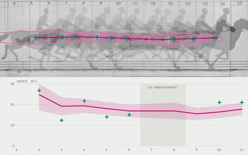
A Kalman filter predicts where the horse will be next (rings, two standard deviations) and then blends the prediction with the measured centroid (cyan crosses); with frames 7 and 8 withheld it coasts on its prediction, and its speed estimate (below) settles near 18 m/s while the frame-to-frame measurements jump between 12 and 27.
A Kalman filter keeps a running best guess of where something is and how fast it is moving, together with how unsure that guess is. Each frame it predicts the next position, then blends that prediction with the new, noisy measurement, trusting whichever is less uncertain. In video tracking it smooths jittery detections and carries a target through a moment when it is hidden.
The machine sees where you're probably going next
In the world Developed for aerospace navigation and guidance, it now smooths tracks in radar, GPS, missile guidance, CCTV people tracking and phone motion sensors.
In art
Ken Goldberg & Gil Gershoni, Are We There Yet?: 5,000 Years of Answering Questions with Questions (2011). A sound installation in the skylit Yud Gallery of the Contemporary Jewish Museum, San Francisco, where recorded questions moved with visitors. The tracking software, described in a paper by Godbehere and Goldberg, subtracts an adaptive background model, groups foreground pixels into connected components, and follows each visitor with 'a bank of Kalman filters'. source
36
Particle filters
CONDENSATION · sequential Monte Carlo · bootstrap filter
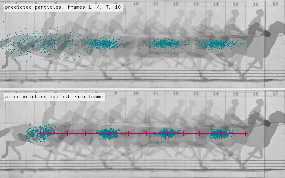
A particle filter tracks with 400 guesses: each step it pushes them forward by their own velocity plus noise (top, a spread of ±84 px at frame 7), weighs each by how much horse silhouette lies in a box around it, and redraws the cloud in proportion to the weights (bottom, ±42 px); the weighted mean (magenta) is the track.
Instead of one best guess, keep hundreds of guesses, called particles, about where the target is. Each frame, move every guess according to a motion model, score it against the image, and resample so good guesses multiply and bad ones die out. Because the cloud of guesses can split, it can follow an outline through visual clutter and keep several hypotheses alive at once, where a Kalman filter keeps only one.
The machine sees a swarm of guesses, thinning toward the truth
In the world Tracking hands, faces and outlines in cluttered video, robot localisation ('where am I on this map?'), and multi-target tracking in surveillance and sports analytics.
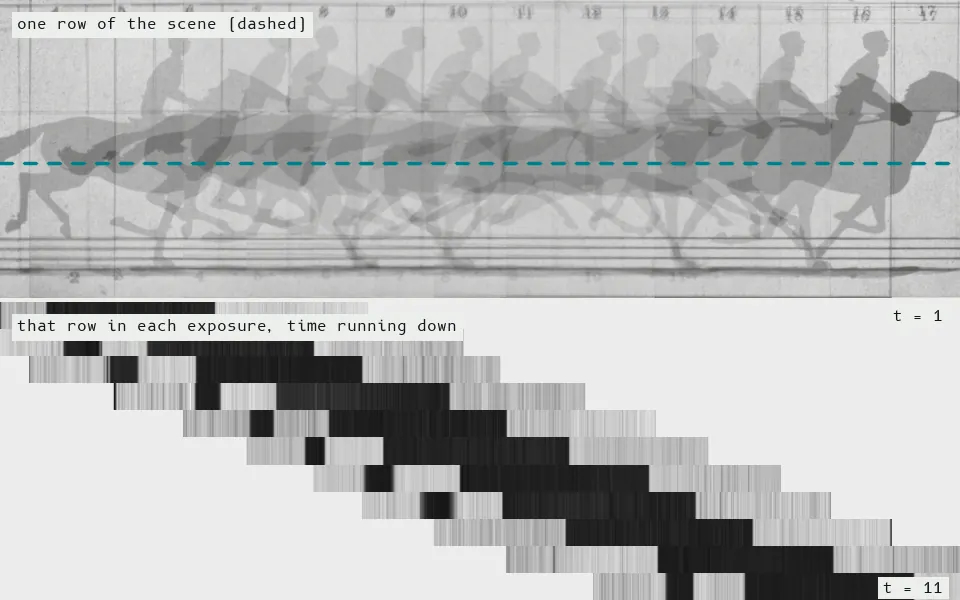
A spacetime slice reads one row of the scene (dashed, through the horse's belly) from each of the eleven exposures and stacks the rows in time order: the still backdrop's ruled lines run straight down, while the horse becomes a band slanting right, its slope a speed, since about 1/25 s separates one row from the next.
Take a single column (or row) of pixels from each video frame and lay the columns side by side. One axis of the result is space and the other is time. Things that stand still become stretched stripes, and things that move smear or warp according to their speed.
The machine sees time laid out as space
In the world Photo-finish cameras at races, line-scan cameras over conveyor belts and inside document scanners, and push-broom satellite sensors that build an image line by line as they pass overhead.
In art
Jussi Ängeslevä & Ross Cooper, Last Clock (2002). It looks like an analogue clock, but its second, minute and hour hands are slices of a live video feed arranged as concentric rings. Each hand 'leave[s] a slitscan video trace' as it circles, so the face fills up with the last minute, hour and twelve hours of whatever passed the camera, 'an ever changing mandala of past'.
38
Temporal median and exposure stacking
frame averaging · image stacking · median background · computational long exposure
No single inventor: long-exposure photography did it on film; a per-pixel median over a stack of frames became a standard way to estimate an empty background, Per-pixel mean or median over a stack of frames from a fixed camera
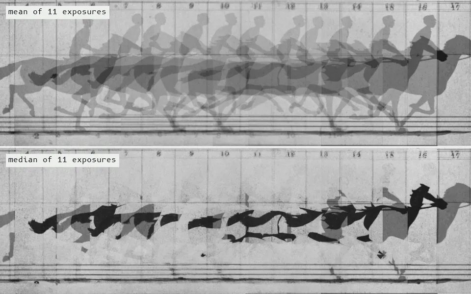
Stacking the eleven registered plates pixel by pixel: the mean (top) is a long exposure in which every pose shows as a ghost, while the median (bottom) keeps only what is present in more than half the exposures, so the riders and legs vanish but the body, which overlaps itself from plate to plate, survives as a dark ribbon.
Line up many frames from a fixed camera and, at every pixel position, take the average or the median of that pixel's values over time. The average blends everything into a ghostly long exposure. The median keeps the value seen most of the time, so passers-by vanish and the empty scene remains. Astronomers and phone night modes stack exposures the same way to cut noise.
The machine sees what stays, with whoever passed through erased
In the world Estimating the empty background for traffic and CCTV analysis, removing tourists from photos of landmarks, and the night and astrophotography modes that stack many frames.
In art
Jim Campbell, Illuminated Average #1: Hitchcock's Psycho (2000). Campbell averaged every frame of Psycho into one still image. His Illuminated Averages series is made by 'averaging all of the frames of a moving sequence.' Because it is a mean rather than a median, the film's figures dissolve into a soft field of light rather than disappearing.
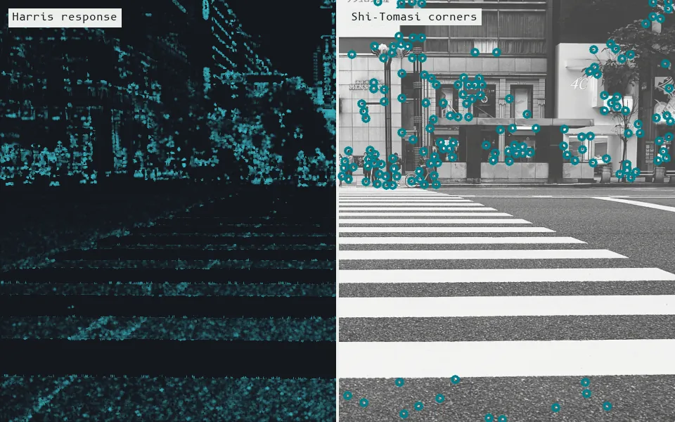
The Harris operator scores every pixel for "cornerness" (left; 1711 local peaks), and Shi-Tomasi keeps the 400 strongest, well-separated corners (right).
A corner detector looks for small patches of an image that change whichever way you nudge them: the tip of a roofline, the corner of a window, a fleck on a rock. Flat areas don't change when shifted, and edges change in only one direction, so the detector scores each pixel by how sharply brightness varies both ways and keeps the top scorers. Harris and Stephens wrote the score in 1988. Shi and Tomasi's 1994 version picks the corners that are easiest to follow from one video frame to the next, which is why OpenCV still calls it 'good features to track'.
The machine sees a scatter of points where edges meet
In the world Corners are the anchor points for video stabilization, visual odometry on robots and drones, and the frame-to-frame tracking under many AR and mapping systems.
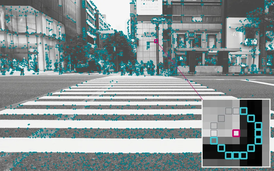
FAST marks 3377 corners by testing a ring of 16 pixels around each point; inset: 11 of the 16 differ from the centre by more than the threshold.
FAST is a corner detector built for speed. For each pixel it looks at a ring of 16 neighbors and asks a yes-or-no question: is there an unbroken run of them that are all much brighter, or all much darker, than the center? Rosten and Drummond used machine learning to choose which ring pixels to test first, so most pixels are rejected after two or three comparisons. That made it practical to find hundreds of corners per video frame on a phone or a small robot's computer.
The machine sees a ring of pixels voting on whether the center is a corner
In the world FAST, often inside ORB, does the corner finding in real-time tracking and SLAM: phone AR, robot and drone navigation, and mapping from moving cameras.
41
Scale-space blobs (LoG, DoG)
Laplacian of Gaussian · Difference of Gaussians · blob detection · automatic scale selection
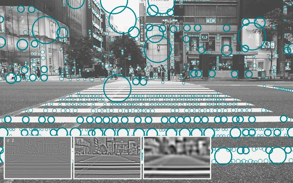
Difference-of-Gaussian filtering finds 649 blobs, each circled at the scale where it responds most; insets show the filtered image at three scales.
A blob detector looks for spots: patches brighter or darker than their surroundings, like a stone in a field, an eye, or a star. It blurs the image at many strengths and compares neighboring blur levels. A spot of a given size responds most strongly at the blur that matches it, so the detector reports both where each blob is and how big it is. Subtracting two blurred copies (the Difference of Gaussians) is a cheap stand-in for the Laplacian of Gaussian, and it is the first stage of SIFT.
The machine sees circles of every size, each fitted to a spot
In the world Blob detectors find spots in microscope and telescope images, and supply the keypoints that SIFT-based mapping and image-search systems match.
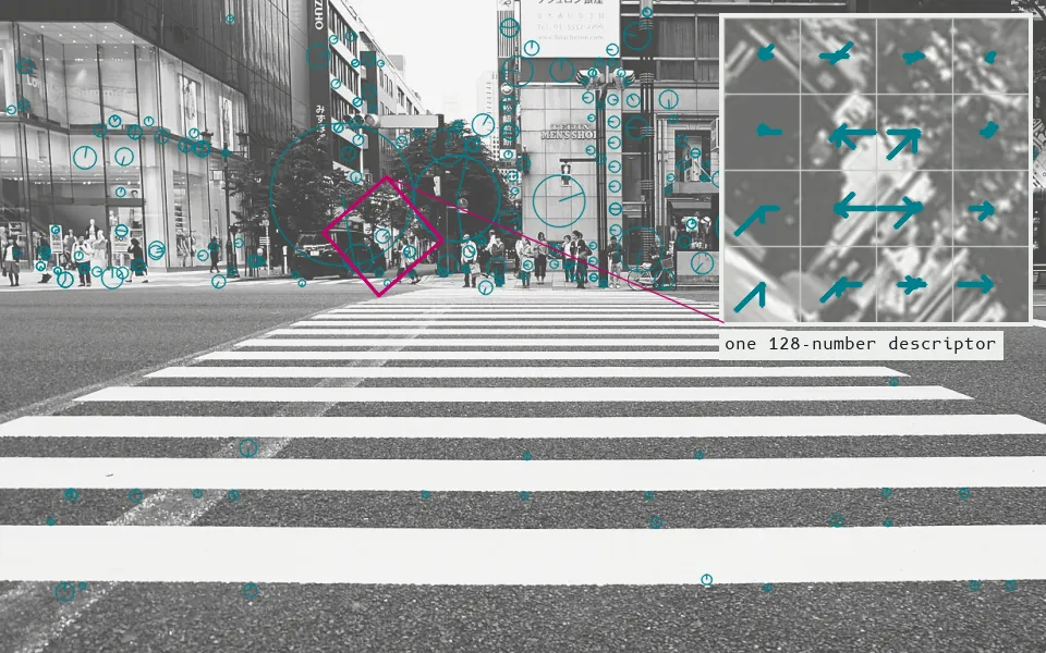
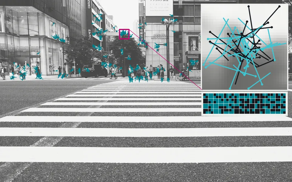
SIFT finds 4492 keypoints, each with a scale (circle) and orientation (strongest 260 shown); inset: one keypoint's descriptor, 8 gradient directions in a 4x4 grid.
SIFT turns an image into a few thousand distinctive points, each with a numerical fingerprint. It finds blobs at every scale (see scale-space blobs), then describes the patch around each one by the directions its edges run, tallied in a small grid of histograms: 128 numbers per point. Because each fingerprint is measured relative to the patch's own size and angle, the same mountain ledge gets roughly the same fingerprint whether the photo is zoomed, rotated or lit differently. Matching fingerprints between two images lets a machine say 'this is the same place' without any idea what a mountain is.
The machine sees thousands of circled keypoints, each reduced to 128 numbers
In the world SIFT-style matching underpins panorama stitching, 3D reconstruction from photo collections, robot localization and image search.
In art
Trevor Paglen, Matterhorn (How to See Like a Machine) Brute-Force Descriptor Matcher; Scale Invariant Feature Transform (2016). Paglen photographed the Matterhorn and ran computer-vision scripts on top of the photographs. The title names the two he used: SIFT, and a brute-force descriptor matcher, which compares every SIFT fingerprint against every other. The result is a mountain overwritten by what the algorithm finds there. It is Fig. 0.1 in How to See Like a Machine.
43
SURF, BRIEF and ORB
Speeded-Up Robust Features · Binary Robust Independent Elementary Features · Oriented FAST and Rotated BRIEF · binary descriptors
ORB finds 500 oriented keypoints; inset: the BRIEF idea behind binary descriptors, where 256 brightness comparisons inside a patch become 256 bits.
SURF (2006), a faster cousin of SIFT, replaces SIFT's careful blurring with box-shaped filters that can be computed almost instantly. BRIEF (2010) and ORB (2011) go further: each point's fingerprint becomes a string of a few hundred yes/no answers to questions like 'is this pixel brighter than that one?'. Comparing two such strings means counting where they disagree, which a phone chip can do millions of times a second. ORB added rotation handling and was free to use, unlike the patented SIFT and SURF.
The machine sees each point reduced to a barcode of brighter/darker comparisons
In the world ORB is the standard feature in open-source visual SLAM (ORB-SLAM) on drones and robots, and binary descriptors run in phone AR and image-recognition apps where SIFT was too slow.
In art
Trevor Paglen, Camel Butte — SURF (Speeded-Up Robust Features) (2020). An albumen print of a Western landscape, overlaid with the marks of the SURF algorithm. For this series Paglen ran modified machine-vision software over his 8x10 negatives and, in the gallery's words, overlaid 'lines, circles and strokes that signify how computer vision algorithms attempt to see', then printed by hand with 19th-century processes. source
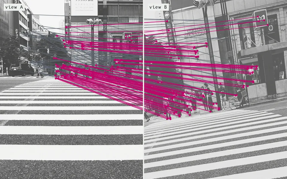
ORB proposes 221 matches between two views of the street; RANSAC keeps the 128 that agree on one homography (magenta) and rejects 93 (grey).
Once two images have been turned into feature points, a matcher pairs each point with the most similar fingerprint in the other image, and many of those pairs are wrong. RANSAC sorts them out by repeated guessing: pick a few pairs at random, work out the camera move or shape change they imply, and count how many other pairs agree. After a few hundred tries it keeps the guess with the most support and discards the rest as outliers. Fischler and Bolles devised it at SRI for automated cartography, working out where a camera was from photos of known landmarks.
The machine sees a tangle of match lines, sorted into the ones that agree and the outliers
In the world Match-then-RANSAC is the checking step in panorama stitching, photo-based 3D mapping, visual navigation, AR tracking, and image search that confirms two photos show the same object.
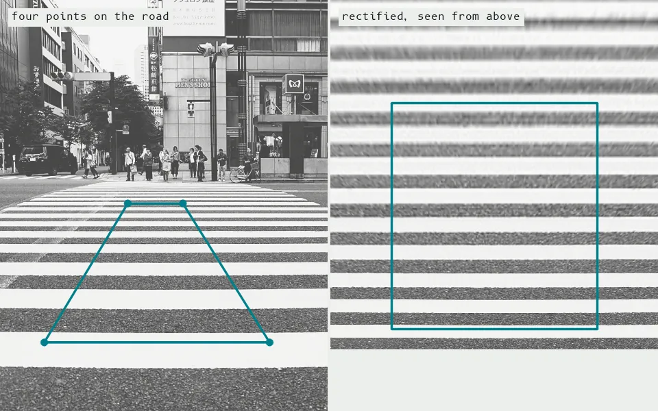
Four points on the road fix a 3x3 homography that re-projects the photograph as if seen from directly above: the converging crosswalk stripes come out parallel and evenly spaced.
A homography is the rule that maps a flat surface seen from one viewpoint onto the same surface seen from another. Four matching points, such as the four corners of a poster in two photos, are enough to compute it, and then every other pixel can be moved to match. It is how software straightens a photo of a document, lines a projector up with a wall, or pastes an image onto a billboard so it looks painted there. It is exact only for flat things; anything that sticks out of the plane gets smeared.
The machine sees every flat surface as a four-cornered shape that can be pulled into any other
In the world Homographies straighten scanned documents and license plates, place broadcast graphics on sports fields, align projectors, and anchor AR content to tables, walls and signs.
In art
Julian Oliver, with Damian Stewart and Arturo Castro, The Artvertiser (2008–). Hand-held binoculars running custom software recognize billboards in the street and replace them, live, with artworks. The software finds the billboard's plane and computes a homography, the perspective warp that lays the substitute image exactly over the ad. Its own source code also uses RANSAC to reject false matches. source
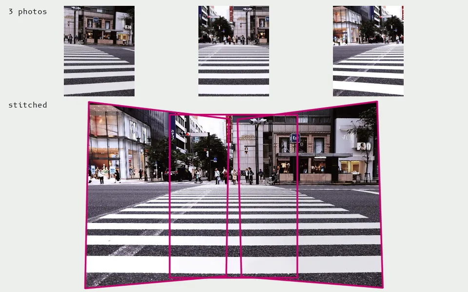
Three overlapping photos (synthesized by rotating a virtual camera within the specimen) are matched with SIFT (420 and 437 RANSAC inliers), warped by homographies and feather-blended into one panorama; magenta shows each frame's footprint.
Stitching merges overlapping photos into one seamless wide image. The software finds matching feature points where neighboring photos overlap, uses them to work out how each camera was turned relative to the others, warps every photo onto a shared surface (a cylinder or sphere for a full panorama), and blends the seams so the joins disappear. When something moves between shots, or sits at a very different depth, the pieces can't agree: people get sliced, cars repeat, roads break.
The machine sees the world as one continuous surface sewn from many glances
In the world Stitching builds Google Street View and other street-level mapping, phone panorama modes, and the satellite and aerial mosaics used for mapping.
In art
Jon Rafman, Nine Eyes of Google Street View (9-eyes) (2008–). Rafman screen-captures scenes found inside Google Street View, whose panoramas come from a nine-lens camera on Google's cars (the 'nine eyes' of the title) and are stitched by software. He doesn't stitch anything himself; he harvests the output, including its failures, such as a pedestrian broken apart by what one critic calls 'the mechanism for reassembling the images'. source
47
Template matching
cross-correlation matching · normalized cross-correlation · scene matching · area correlation
Daniel Barnea & Harvey Silverman (an early classic; correlation matching was in use before them), 1972, A Class of Algorithms for Fast Digital Image Registration (IEEE Transactions on Computers, 1972)
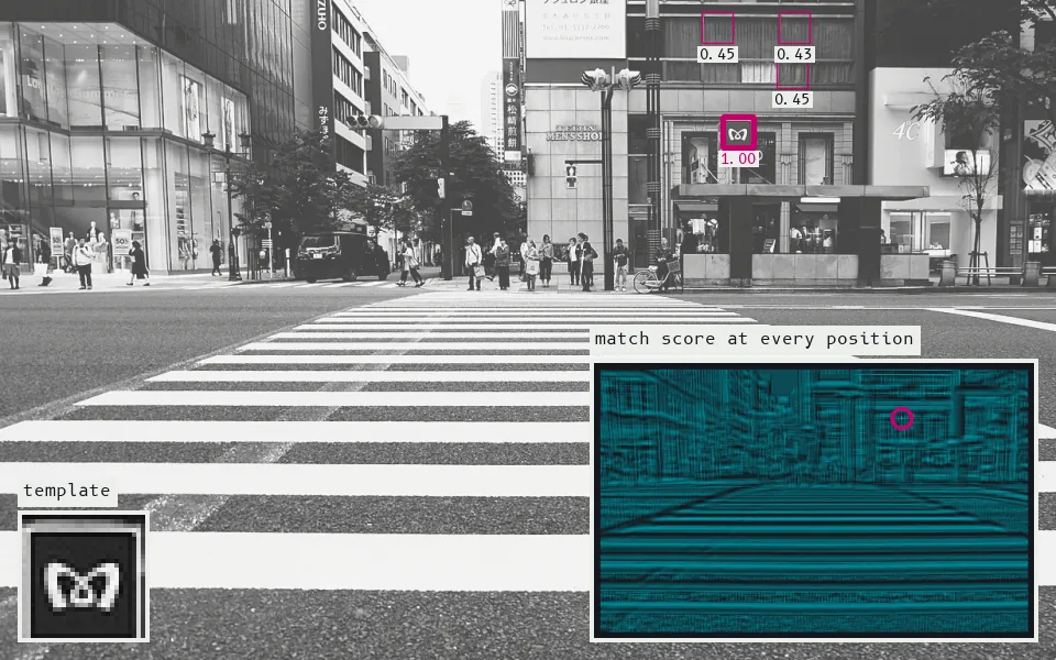
A 28x28-pixel template (the subway sign) is compared with every position by normalized cross-correlation (inset, bright = similar); it scores 1.00 where it was cut, and the next-best place only 0.45.
Template matching is the most literal way to find something: take a small reference picture (the template), slide it across a bigger image, and score how well it lines up at every position. The best score marks where the thing is. It needs no training and no features, but it only works if the target looks almost exactly like the template: same size, same angle, same lighting.
The machine sees a heat map of how closely each spot resembles a stored picture
In the world Stored-scene matching guides cruise missiles onto targets (the Tomahawk's DSMAC compares a stored image of the target with the live view), and template matching still checks parts on factory lines and locates on-screen elements for software bots.
In art
Harun Farocki, Eye/Machine III (2003). The third part of Farocki's Eye/Machine cycle, built around his idea of the 'operational image', an image that is part of a process rather than a picture of one. Its central example is the 1980s cruise missile that 'used a stored image of a real landscape then took an actual image during flight, the software compared the two images': template matching as weapon guidance, which Farocki reads as a montage of 'similarity and difference'.
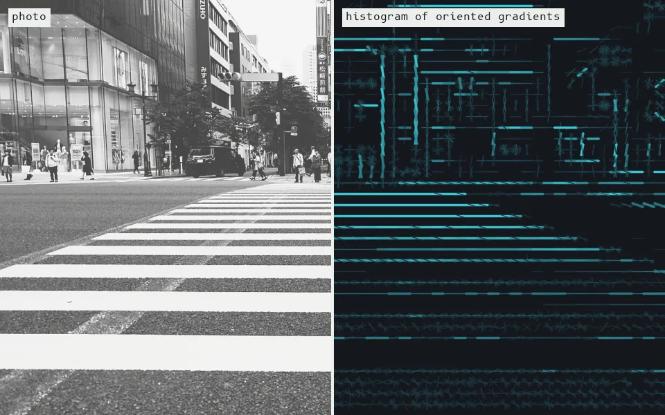
HOG divides the image into 60x37 cells of 16 pixels and records how much edge runs in each of 9 directions; the right half shows each cell as a star of those edges.
HOG describes the shape of a region by the directions of its edges. It divides an image window into small cells, measures which way brightness changes at each pixel, and tallies those directions into a little histogram per cell, adjusted against neighboring cells so lighting matters less. The result is a coarse sketch of where edges run. Paired with a simple linear classifier, it became the standard way to find people in photos in the late 2000s.
The machine sees a grid of tiny compass roses tracing where edges point
In the world HOG with a support vector machine was the go-to pedestrian detector in driver assistance and CCTV analytics before deep learning, and dlib's widely used face detector is HOG-based.
49
Bag of visual words
bag of features · bag of keypoints · visual vocabulary · Video Google
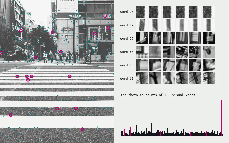
873 SIFT descriptors are clustered into a vocabulary of 100 visual words (rows: patches assigned to six of them), and the whole photo becomes a histogram of word counts, ignoring where anything is.
This method borrows a trick from text search. Feature fingerprints (such as SIFT) from thousands of images are clustered into a few thousand typical patterns, the 'visual words'. Each image is then described only by how often each word occurs, ignoring where. A picture becomes a word-count list, so image search can reuse the indexing and ranking that search engines use for documents, and a classifier can learn which word counts mean 'car' or 'face'.
The machine sees a picture as a shuffled bag of a few thousand stock fragments
In the world Visual words powered large-scale image and video retrieval, landmark recognition, and the place-recognition step that lets robots and drones notice they have returned somewhere (as in ORB-SLAM).
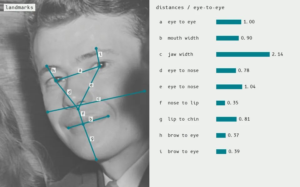
In Bledsoe's method, an operator marked points on a photo and the machine compared distances between them; here 11 points located by a landmark model become 9 numbers, scaled by the eye-to-eye distance.
A face becomes a list of measurements. An operator marks key points on a photo (pupils, corners of the eyes, tip of the nose, corners of the mouth), and the computer records the distances between them. To identify someone, it compares that list with the lists stored for known faces and returns the closest. Bledsoe corrected for tilted and turned heads by fitting each face to an average "standard head" (Fig. 5.7 in the book).
The machine sees a face as a list of distances between points
In the world Landmark points are still how most face systems line a face up before matching it, from phone unlock to passport e-gates, and the first version was paid for by the CIA through a front company.
In art
Zach Blas, Face Cages (2014–16). Blas and three other queer artists (micha cárdenas, Elle Mehrmand, Paul Mpagi Sepuya) generated the point-and-line biometric diagrams of their own faces and had them fabricated in stainless steel as cages, which they wore in endurance performances.
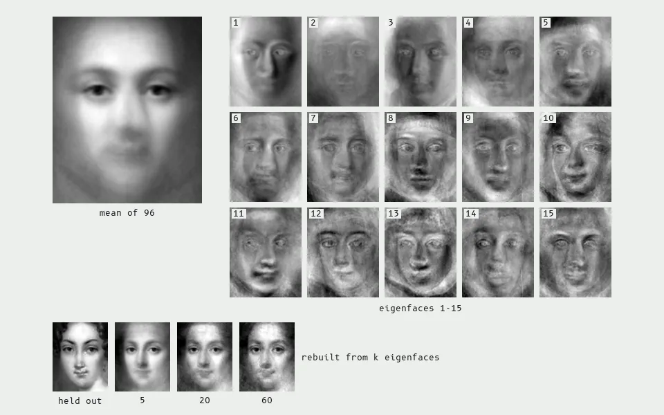
Eigenfaces of 96 aligned faces from Met portrait paintings: the mean face, the first 15 principal components (together the first 10 explain 71% of the variation), and a held-out portrait rebuilt from 5, 20 and 60 of them.
Given many aligned photos of faces, the method finds a small set of "ingredient" images, the eigenfaces, that can be mixed in different amounts to rebuild any face in the set. Each face then becomes a short list of mixing amounts, and recognition compares those lists. The eigenfaces look like ghostly, blurred faces, and the book (Ch. 1) describes the leftover individual pattern as a facial "fingerprint."
The machine sees a face as a recipe of ghost faces
In the world Eigenface matching was among the methods tested in FERET, the 1990s US military-funded face-recognition benchmark, and was an early basis for commercial face recognition.
In art
Trevor Paglen, "Fanon" (Even the Dead Are Not Safe) Eigenface (2017). Paglen ran face-recognition software on photographs of Frantz Fanon and printed the resulting eigenface (the machine's averaged 'faceprint' of him) as a large portrait. It is Fig. 1.3 in the book. source
52
Fisherfaces
linear discriminant analysis (LDA) for faces · Fisher linear discriminant
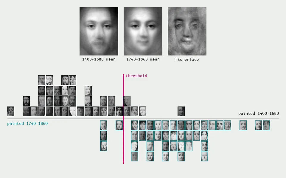
Fisherfaces look for the one face-direction that best separates two labelled groups, here 47 Met portraits painted 1400-1680 and 50 painted 1740-1860; projecting onto it sorts 81 of 97 correctly (leave-one-out), on fashion and painting style as much as on faces.
Like eigenfaces, it reduces each face to a few numbers, but it chooses them differently. Eigenfaces keep whatever varies most across all photos, which is often lighting. Fisherfaces keep the patterns that best separate one person from another while ignoring the changes that happen to the same person (light, expression). Each face becomes a point placed to push different people apart.
The machine sees a face as only the differences that tell people apart
In the world Fisherfaces was a standard face-recognition method in 2000s research and still ships in OpenCV's face module, so it turns up in low-cost door-access and classroom-attendance systems.
In art
Rafael Lozano-Hemmer, Level of Confidence (2015). A webcam installation trained on photographs of the 43 students disappeared from the Ayotzinapa teachers' college in Iguala, Mexico. It compares each visitor's face with theirs using the Eigen, Fisher and LBPH face-recognition algorithms and shows the closest student with a 'level of confidence' percentage.
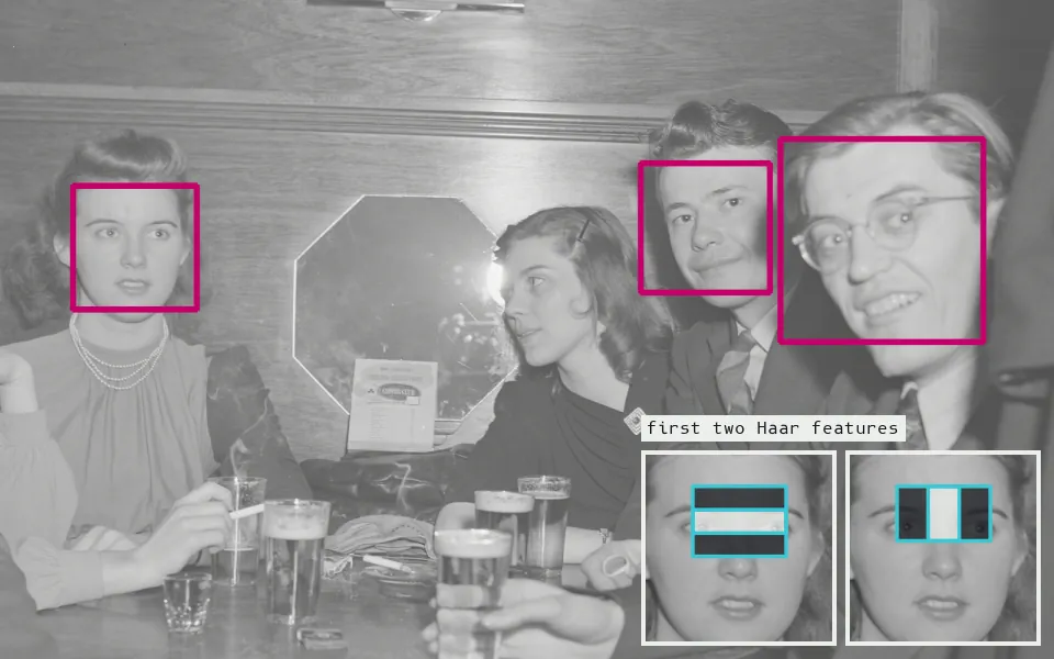
A Viola-Jones cascade finds 3 faces (the head turned away is missed); insets: its first two tests compare light and dark rectangles, eyes darker than cheeks and nose bridge lighter than eyes.
A small window slides over the image at every position and size, asking a chain of quick questions about light and dark rectangles: are the eyes darker than the cheeks? Is the bridge of the nose brighter than the eyes? Most windows fail within a question or two and are thrown out; only windows that pass every stage (OpenCV's standard face cascades have about 20–25) are called faces. That speed made real-time face detection possible on 2000s cameras.
The machine sees a face as a pattern of light and dark boxes
In the world Haar cascades drew the face boxes in 2000s digital cameras and webcams and were the first step in many recognition and crowd-counting systems, since a face has to be found before it can be recognized.
In art
Adam Harvey, CV Dazzle (2010). Harvey designed hair and makeup looks whose bold dark and light patches reverse the light-dark pattern the Haar cascade expects around the eyes, nose bridge and cheeks, so OpenCV's Viola–Jones detector fails to find a face.
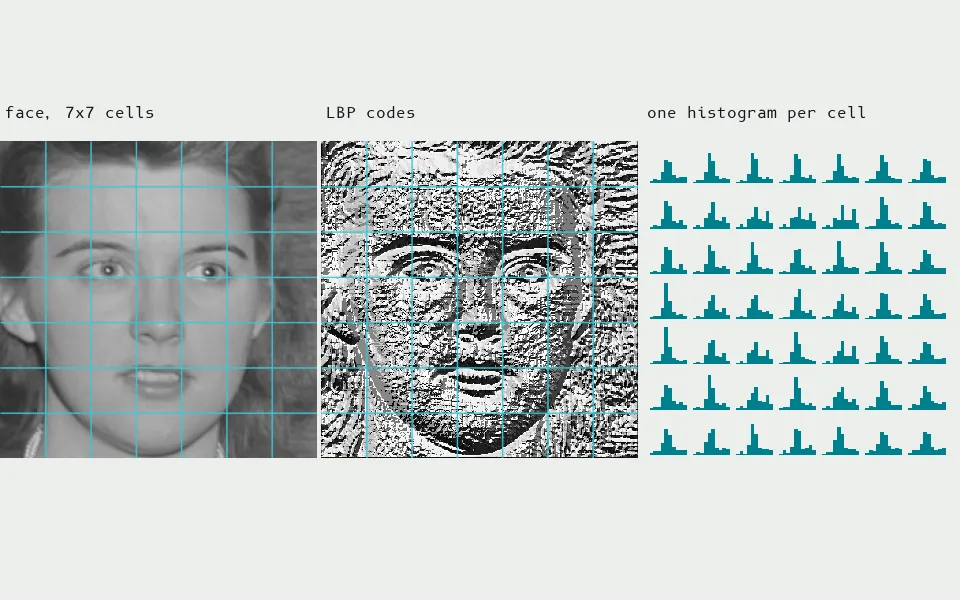
Local binary patterns rewrite each pixel as an 8-bit code (is each neighbour brighter?); the face becomes 49 histograms of those codes, one per cell, which is what an LBP face recognizer compares.
Each pixel is compared with its eight neighbors: a 1 where the neighbor is brighter, a 0 where it is darker. The resulting 8-digit code names the tiny texture at that spot (an edge, a corner, a spot, a flat patch). Counting the codes in each patch of a face turns the face into a stack of histograms, and two faces are compared by comparing histograms. Because it only asks "brighter or darker?", it is largely unbothered by overall lighting.
The machine sees a face as a census of tiny textures
In the world LBP was a cheap, lighting-tolerant choice for face matching and 'is this a live face or a printed photo?' checks on low-power hardware, and OpenCV ships both an LBP face recognizer and LBP face detectors.
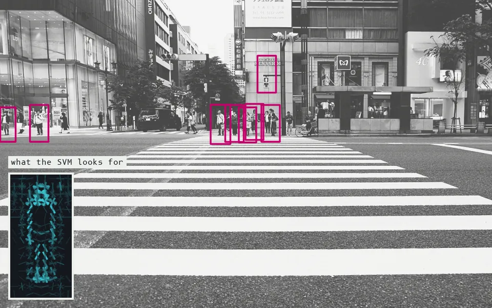
Dalal and Triggs's HOG-plus-SVM detector, scanning the photo at 2x, reports 8 people (magenta), one of them a pedestrian traffic signal; inset: the detector's positive weights drawn as edges, a standing figure outlined in 3,780 numbers.
A tall, person-shaped window is divided into small cells, and in each cell the method records which way the edges point (a histogram of oriented gradients), giving a rough sketch of a body's outline. A linear classifier (a support vector machine) trained on thousands of cropped photos of people and non-people scores that sketch. Sliding the window across the image at many sizes finds upright people.
The machine sees a person as an upright bundle of edge directions
In the world Detectors of this kind were the standard for spotting pedestrians in driver-assistance research and for counting people in CCTV and retail footfall analytics until neural networks replaced them in the 2010s.
56
Active shape and appearance models
ASM · AAM · constrained local models (CLM) · deformable face models · FaceTracker
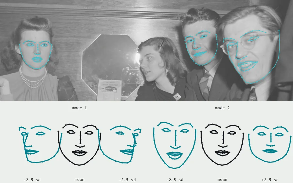
A shape model in the manner of Cootes's Active Shape Models: PCA over 68-point landmark sets from 97 Met portraits gives the mean face shape and its main modes of variation (84% and 5%, below); above, OpenCV's LBF facemark fits the same 68 points to the 1941 photograph.
A face is modeled as a mesh of about 60–70 points learned from hand-labeled photos, together with the ways that mesh is allowed to bend (smiling, opening the mouth, turning the head). To track a face, the mesh is placed on the image and each point is nudged toward the edge or texture it expects, while the whole shape is kept face-like. Appearance models also learn the texture inside the mesh, so they can redraw the face.
The machine sees a face as a flexible wireframe of points
In the world Trackers in this family powered early face filters and avatar animation, driver-drowsiness and expression analysis, and they align faces before matching in recognition systems.
In art
Kyle McDonald & Arturo Castro, Face Substitution (2011). Real-time face tracking fits a deformable mesh to the viewer's face and pastes another person's face onto it, so it moves with their expressions. The code is built on ofxFaceTracker, McDonald's wrapper for Jason Saragih's FaceTracker. source
57
Skin-color detection
skin segmentation · flesh-tone detection
Michael Jones & James Rehg, 1999, Statistical Color Models with Application to Skin Detection (CVPR 1999; IJCV 2002)
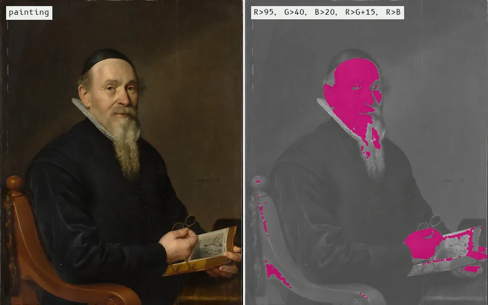
A fixed colour rule (Peer and Kovac, 2003) marks 6% of pixels as skin, the face and hands but also the warm wood of the chair; the 1941 photo has no colour, so this figure uses a painting.
Each pixel is labeled skin or not-skin by its color alone, using a lookup table built from millions of hand-labeled pixels or a simple rule such as a range of hues. The result is a mask of skin-colored blobs, used to find faces and hands quickly or to flag pictures with a lot of exposed skin. Because "skin" is learned from whatever photos were labeled, it can fail on some skin tones and fire on wood, sand and other skin-colored things.
The machine sees the world as skin-colored or not
In the world Skin detectors were an early filter for nudity in web and image-search filtering and a fast first step for finding hands and faces in webcams and gesture interfaces.
John Merchant, Richard Morrissette & James Porterfield (Honeywell), 1974, Remote Measurement of Eye Direction Allowing Subject Motion Over One Cubic Foot of Space (IEEE Trans. Biomedical Engineering)
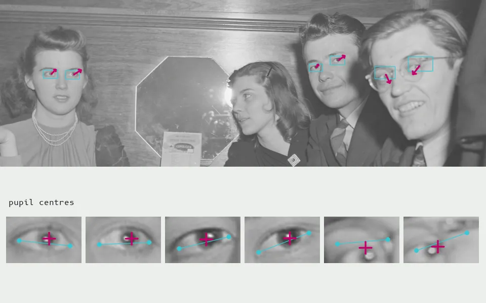
For 6 eyes on 3 detected faces, the pupil is located as the point that image gradients radiate from (Timm and Barth, 2011), and its offset from the middle of the eye corners gives a gaze direction (magenta, exaggerated 5x); behind the glasses at right the estimates are least certain.
An infrared light shines on the eye, so the pupil shows up as a sharp dark (or bright) disk and the cornea reflects a small glint. Software finds the pupil's center, typically by thresholding and fitting an ellipse, and measures its offset from the glint. After a short calibration in which the person looks at known points, that offset is mapped to where they are looking.
The machine sees an eye as a dark disk and a bright dot
In the world Gaze trackers run in advertising and usability labs, in assistive devices for people who cannot move, and in the driver-monitoring cameras that check whether truck and car drivers are watching the road.
In art
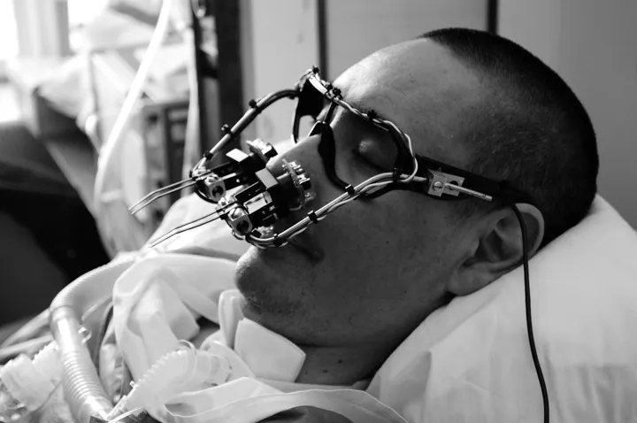
Zach Lieberman, James Powderly, Evan Roth, Chris Sugrue, Theo Watson, with Tony Quan (TEMPT1), The EyeWriter (2009). Low-cost glasses with a hacked PlayStation Eye camera, infrared filters and infrared LEDs film the eye, and custom openFrameworks software turns its movements into drawing, letting TEMPT1, a graffiti artist paralyzed by ALS, tag buildings with projected light.
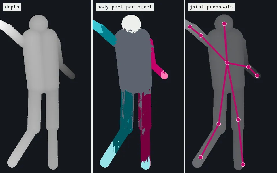
A synthetic depth image (a diagram of the Kinect method, no camera involved): a random forest trained on 60 rendered poses labels each pixel as one of 10 body parts from depth differences alone (81% of pixels correct), and part centres become a skeleton.
A depth camera such as the Kinect measures how far away each pixel is, so a person stands out from the room as a 3D silhouette. Shotton's method labels every depth pixel with a body part (left hand, right knee, head) using a randomized decision forest trained on about a million computer-generated depth images of people in different poses, then places a joint at the center of each part. The output is a stick-figure skeleton, 30 times a second, with no markers or suits.
The machine sees a body as a stick figure in depth
In the world Kinect skeleton tracking shipped in millions of Xbox consoles and was quickly repurposed for physiotherapy, retail analytics, robotics and interactive installations.
In art
Design I/O (Theo Watson & Emily Gobeille), Puppet Parade (2011). Two Kinect depth cameras track the arms of children standing in front of the screen, and their arm movements puppeteer large projected creatures.
A diagram of classic finger counting: on six synthetic hand silhouettes, the deep dents between the outline and its convex hull (cyan dots) are counted, and the count (magenta) is right for 5 of 6 poses.
A movement (a finger on glass, a tracked hand, a mouse) is recorded as a path of points. The $1 recognizer resamples that path to a fixed number of points, rotates and scales it to a standard size, and compares it point by point with stored templates such as a circle, a check mark or a zigzag; the closest template wins. Camera-based systems first find the hand (often by skin color or depth) and then classify its path or shape the same way.
The machine sees a movement as a line to match against templates
In the world Gesture recognition runs swipe shortcuts on touchscreens, motion controls on game consoles and car dashboards, and hand-tracking interfaces in VR headsets.
In art
Myron Krueger, Videoplace (1969–75 (developed through the 1980s)). A camera digitizes the participant's silhouette against a backlit wall, and the system analyzes its posture, shape and gestural movements, so that visitors can draw with their fingers, 'shoot' with a pointed finger, or watch a graphic critter climb their projected silhouette. source
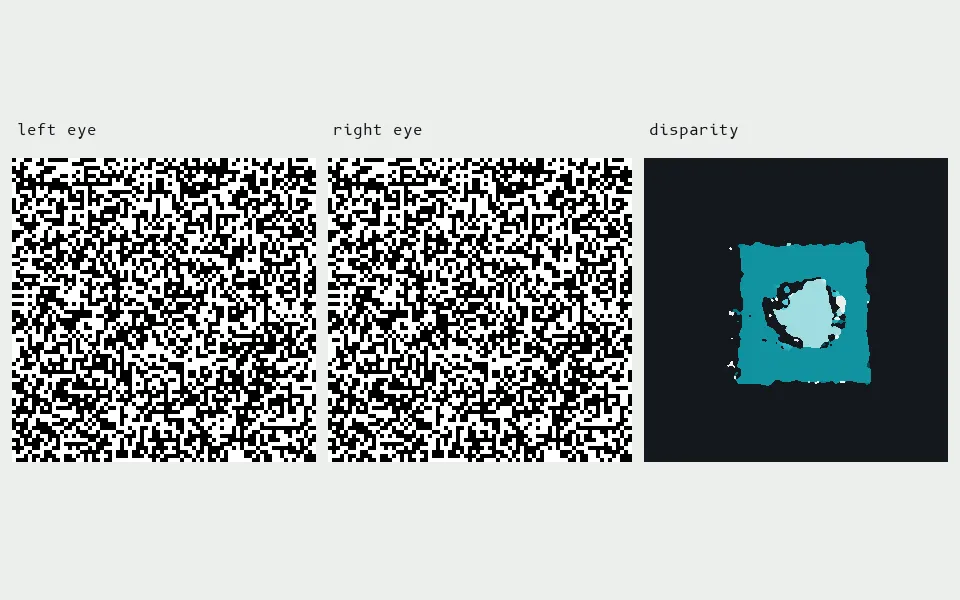
A random-dot stereogram after Julesz (1960): neither image alone contains a shape, but semi-global block matching finds a square shifted 3.0 dots (true: 3) and a disc in front of it (true: 6) between the two views.
Two cameras a short distance apart see the world from slightly different positions, so nearby things shift more between the two images than distant ones. Stereo software finds, for each point in the left image, the matching point in the right image; the size of that shift (the disparity) gives the distance. The hard part is the matching: which dot goes with which. Julesz's random-dot pictures showed that human vision solves it without recognizing any objects, and Marr and Poggio wrote an algorithm that did the same.
The machine sees a depth map where brightness means nearness
In the world Stereo cameras give depth to driver-assistance systems, planetary rovers, warehouse robots and drones, and stereo pairs from satellites and aircraft are how elevation maps are made.
In art
Béla Julesz, Random-dot stereograms in 'Computer-Generated Pictures' (with A. Michael Noll), Howard Wise Gallery, New York (1965). Julesz, a Bell Labs perception researcher, showed computer-generated random-dot patterns as gallery works. Eight were stereo pairs, mounted as polarized left- and right-eye images and viewed through glasses supplied at the gallery, so a hidden shape floated out of the noise. They are depth from disparity alone, with no other cue, and random-dot stereograms like these became the standard test for computational stereo.
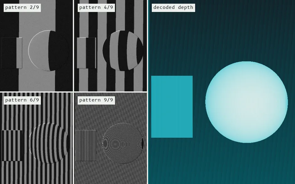
Structured light, simulated: a projector beside the camera throws 9 Gray-code stripe patterns (four shown) that bend over a sphere and a box; decoding the on/off sequence at each pixel gives the projector column, and triangulation gives depth (median error 1.0 cm).
Structured light measures shape by projecting a known pattern (a line, stripes, a grid or a field of dots) onto a scene and filming how it bends. A camera set off to one side sees the pattern shift wherever the surface comes forward or falls back, and triangulation turns that shift into distance. Projecting a sequence of black-and-white stripe codes lets every projector pixel be identified separately, which gives dense, accurate scans of faces and objects at close range.
The machine sees a surface known only by how a projected pattern deforms across it
In the world Structured light runs 3D face unlock on phones (Face ID's dot projector), the first Microsoft Kinect, factory inspection, and dental and body scanners.
In art
Radiohead; directed by James Frost, with Aaron Koblin, House of Cards (music video) (2008). Made with no cameras or lights. Close-ups of Thom Yorke, the female lead and partygoers were captured with Geometric Informatics' structured-light scanner, which records faces as moving clouds of 3D points; the wide and exterior shots came from a Velodyne lidar. The data and code were then released for fans to re-render. source
63
Time-of-flight and LiDAR
lidar · laser scanning · laser rangefinding · ToF camera · point cloud
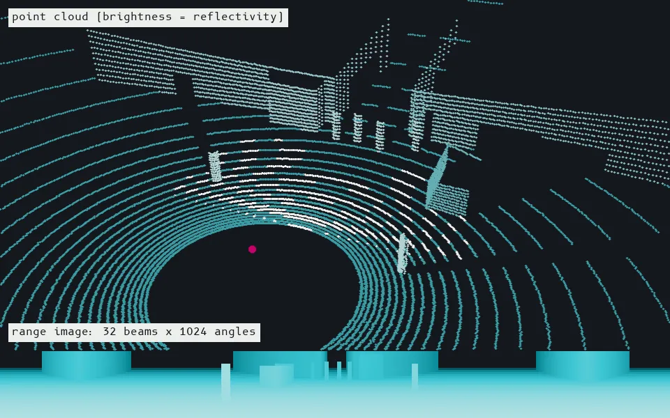
A simulated 32-beam spinning LiDAR (a diagram, not a real scan): each of 29,577 returns is a laser pulse's round-trip time turned into distance, and the strength of the echo picks out the painted crosswalk on the flat road.
Time-of-flight sensors measure distance by timing light. A laser pulse, or a rapidly flickering light, goes out, bounces off a surface and comes back; because light's speed is known, the delay gives the range. A lidar sweeps or spins its lasers to collect millions of these ranges a second, building a point cloud: a 3D scatter of measured dots with no colour or texture of its own. A time-of-flight camera takes a range at every pixel at once.
The machine sees a point cloud: the world as millions of measured dots
In the world Lidar is the main 3D sensor on self-driving cars and delivery robots, maps terrain and forests from aircraft, and scans crime scenes and buildings; time-of-flight cameras sit in phones and in the second-generation Kinect.
In art
Liam Young, written by Tim Maughan, Where the City Can't See (2016). Billed as the first fiction film shot entirely with laser scanners, 'the same scanning technologies used in autonomous vehicles'. A robot-managed Detroit is seen only as the scanners record it, as point clouds, while young factory workers in anti-facial-recognition masks drift through it in a driverless taxi. source
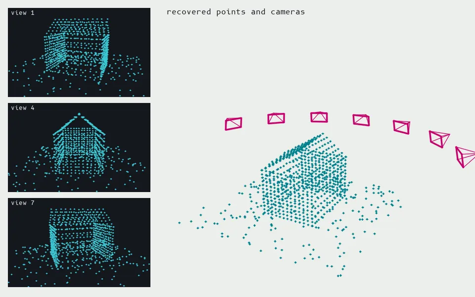
Structure from motion on a synthetic house seen from 7 viewpoints (a diagram): the essential matrix, PnP and a simple bundle adjustment recover every camera (magenta) and 929 points, to 0.64 px reprojection error and 0.5 cm median 3D error once the unknowable scale is fixed.
Structure from motion builds a 3D model out of ordinary photographs taken from different places. It finds matching feature points across the photos, then solves at once for where each camera stood and where each matched point sits in space, adjusting everything until the geometry agrees (bundle adjustment). Dense methods then fill in millions more points and a textured surface. Photo Tourism (2006) showed it could work on thousands of strangers' tourist photos pulled from the internet.
The machine sees a cloud of points floating where the cameras agreed something was
In the world SfM photogrammetry turns drone, aerial and phone photos into 3D maps and city models, records heritage sites and crime scenes, and reconstructs events in open-source investigations.
In art
Forensic Architecture, with Yazda, Maps of Defiance (UK Pavilion, XXII Triennale di Milano) (2019). To record Yazidi villages and shrines in Sinjar, Iraq, destroyed by ISIS in 2014, Forensic Architecture trained local documentation teams to photograph sites with kites, drones and improvised 'bottle rigs'. The thousands of images from each site were processed into geolocated 3D point clouds by structure-from-motion photogrammetry, precise enough to measure how far debris was thrown and so locate the source of an explosion.
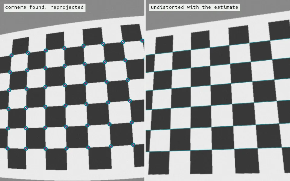
Camera calibration from 9 synthetic views of a chessboard: Zhang's method recovers focal length 700 px (true 700) and barrel distortion k1 = -0.30 (true -0.30), reprojecting the corners to within 0.28 px; undistorting straightens the rows.
Calibration works out a camera's private geometry: its focal length, where its optical center falls, how its lens bends straight lines, and, when needed, exactly where it sits and points. The usual method, from Zhang (2000), is to show the camera a printed checkerboard from several angles; because the software knows the squares are equal and straight, it can solve for whatever distorted them. Without calibration a camera only takes pictures. With it, each pixel becomes a measured ray into the world, which every 3D, tracking and mapping system depends on.
The machine sees every pixel as a ray pointing into the world
In the world Every stereo rig, lidar-and-camera pair on a self-driving car, sports-tracking system, projection-mapping show and photogrammetry survey is calibrated before it measures anything.
In art
Kyle McDonald and Jonas Jongejan, Light Leaks (2013). Fifty mirror balls scatter light from several projectors across a whole room. To control where each reflected dot lands, the artists calibrate the setup: a camera photographs a series of projected structured-light patterns, a reference photo of the room is aligned to a measured 3D model, and from these the software computes where every projector pixel ends up in space. source
Shape from shading on a synthetic relief (a diagram): from one shaded image and the light direction, Pentland's linear method solves for depth (correlation with the true relief 0.88); the streaks run along the light direction, where this method is blind.
Shape from shading recovers 3D shape from a single photo by reading its light and shadow. If you know where the light comes from and assume the surface is evenly matte, how bright each point is tells you how steeply it tilts away from the light, and joining those slopes gives a surface. Real scenes rarely meet the assumptions, so the method has to guess, and a dent lit from below can read as a bump, the same ambiguity that fools human eyes.
The machine sees brightness read as slope
In the world Shape from shading (photoclinometry) maps slopes on the Moon, Mars and asteroids from orbital images; its multi-light cousin, photometric stereo, inspects surfaces for tiny defects in factories.
MSER proposes 216 letter-like regions (cyan), most of them not text; the sign (composited for this figure) is found by its four corners, rectified, and Tesseract reads "LOOK BOTH WAYS" (mean confidence 97).
The page image is split into lines, words and single characters. Each character shape is then matched against known letters: first by comparing it with a stored stencil of each letter (Tauschek's machine did this with light and a mechanical template), later by measuring features such as loops, strokes and endpoints and feeding them to a trained classifier. A dictionary or language model then corrects unlikely guesses.
The machine sees a page as a string of best-guess characters
In the world OCR sorts mail by address, reads checks for banks and passports at border gates, and turned millions of library books into searchable text, often with errors no human reader would make.
In art
Karen ann Donnachie & Andy Simionato, The Library of Nonhuman Books (2019–). A custom reading machine photographs each page of a book with two cameras, runs OCR to turn it into text, then uses language software to keep a few words as a short poem, erase the rest and add a found illustration, and publishes the result as a print-on-demand book with no human editing. source
OpenCV's QR reader finds the three square finder patterns, unwarps the 25x25 grid of modules (inset), samples each one as a bit and decodes "SEE LIKE A MACHINE"; the code was generated and composited onto the wall for this figure.
These are images made for machines to read. A linear barcode is read along one line: the reader measures the widths of the black and white bars and turns them into digits, with a check digit to catch misreads. A QR code is two-dimensional: three square 'finder' patterns in its corners let a camera locate and straighten it, and a grid of black and white cells is read as bits, with enough built-in redundancy that up to 30% of the code can be damaged and still read.
The machine sees black and white as ones and zeros
In the world Barcodes track almost every product through warehouses and checkouts, and QR codes route people to payments, menus, boarding passes and vaccine certificates.
In art
Golan Levin & Asa Foster III (for F.A.T. Lab), QR Codes for Digital Nomads: QR_STENCILER and QR_HOBO_CODES (2011). QR_STENCILER converts any QR code into a laser-cuttable stencil, relying on the code's error correction to tolerate the thin bridges a stencil needs; QR_HOBO_CODES is a set of 100 stencils that port 19th-century hobo signs ('dangerous dog', plus new ones like 'hidden cameras') into machine-readable street markings.
Three ArUco markers (composited onto the road for this figure) are found and identified (ids 7, 23, 42) from the 4x4 bit pattern inside each black square, and their four corners (cyan) are what a robot or AR system uses to work out its pose.
A fiducial is a printed symbol designed to be found easily by a camera: a thick black square with a pattern inside, or a nest of black and white blobs. Software turns the camera image into pure black and white, looks for shapes with the marker's structure, reads the ID encoded in it, and from the way the shape is distorted works out exactly where the marker is and which way it is turned. That lets a computer attach graphics, sounds or instructions to a physical object.
The machine sees objects as numbered tags with a position and an angle
In the world Fiducial tags guide warehouse robots and drones, anchor augmented-reality graphics, and calibrate cameras in film motion capture and factories.
In art
Sergi Jordà, Martin Kaltenbrunner, Günter Geiger & Marcos Alonso (Music Technology Group, Universitat Pompeu Fabra), Reactable (2005). A tabletop synthesizer: players place and turn blocks whose undersides carry fiducial markers, a camera under the translucent table reads each marker's identity, position and rotation with reacTIVision, and those readings set the sound modules and their parameters. source
A synthetic plate on the parked car (about twice real size): a top-hat filter proposes 15 bright plate-shaped regions, the one with the most strokes wins, and its 4 characters, 24x12 pixels in all, are cut apart and matched to font templates, reading "1941".
A camera, usually lit by infrared so the reflective plate glows, captures each passing car. Software finds the plate's rectangle, straightens it, splits it into characters and reads them with OCR. The plate number is stored with the time and place and checked against 'hotlists' of wanted or uninsured vehicles.
The machine sees a car as a string of characters, a time and a place
In the world Plate readers on highways, toll roads, parking garages, police cars and repossession trucks log billions of sightings, the metadata that Paglen (Ch. 1) shows turning into police and commercial revenue.
In art
Kate Bertash (published in 2019 as Kate Rose), Adversarial Fashion (2019). A clothing line printed with fake license plates, designed and tested against OpenALPR and mobile plate-reader products, so that readers log the garments as cars, stamped with a time and place, and junk data enters the same databases as real plates.
Nearest-neighbour classification (k = 7), drawn as a diagram: each pixel of the crosswalk photo becomes a point (brightness, texture), and a new point takes the majority label of its 7 closest training points; 83% of held-out pixels are labelled correctly.
There is no training: the system simply stores every labeled example. To classify something new, it finds the k stored examples most similar to it and takes a vote. Everything depends on how 'similar' is measured and on what was stored, so the method is only as good, and as biased, as its collection.
The machine sees a thing as the company it keeps
In the world Nearest-neighbor search is how face-recognition and reverse-image-search systems find the closest match in a database of millions of faces or photos.
In art
Kyle McDonald, Sharing Faces (2013). Cameras in Anyang, Korea and Yamaguchi, Japan tracked each visitor's face position, pose and expression, and the installation answered with the stored photo of a past visitor in the other city whose face measurements were closest, a nearest-neighbor lookup over more than 50,000 images. source
Rosenblatt's perceptron, drawn as a diagram: on the same pixel data it nudges a straight line after each mistake (1865 corrections over 20 passes; earlier lines in grey) and ends with a single linear boundary that labels 81% of held-out pixels correctly.
Every input pixel is multiplied by a weight, the results are added up, and if the total passes a threshold the answer is 'yes.' Training nudges the weights after each mistake. The result is a straight line (in many dimensions, a flat plane) dividing all possible images into two sides. Rosenblatt's Mark I Perceptron (1960) did this in hardware, with 400 photocells learning to tell simple shapes apart.
The machine sees an image as a weighted sum, above or below a line
In the world Linear classifiers still make the final decision at the end of most vision systems, including deep networks, and score everything from spam to credit risk.
In art
Trevor Paglen, "Stealth Bomber," Linear Classifier (2017). The title names the technique; it belongs to Paglen's 2017 series of images made with and for machine-vision software (shown in A Study of Invisible Images) and appears as Fig. 1.1 in the book. No published description of its production was found.
A support vector machine with an RBF kernel, drawn as a diagram: the curved boundary is defined by 151 of the 320 training points (ringed), the ones nearest the other class; it labels 84% of held-out pixels correctly.
Like a perceptron, an SVM draws a boundary between two classes, but it picks the boundary that leaves the widest possible gap between them. That boundary is fixed only by the hardest, closest examples, the 'support vectors.' A mathematical shortcut, the 'kernel trick,' lets it draw curved boundaries too. Through the 2000s the standard recipe for recognizing things was hand-designed features (HOG, SIFT, bags of visual words) fed into an SVM.
The machine sees categories as two sides of the widest possible gap
In the world SVMs made the final call in 2000s pedestrian detectors, image-search and object-recognition systems, and they are still used where data is scarce, from medical imaging to factory inspection.
In art
Christian Möller, Cheese (2003). Six actresses held a smile for up to an hour and a half while an emotion-recognition system scored it; when the smile's 'sincerity' dropped below a threshold an alarm sounded. The system was based on the expression-recognition research of UCSD's Machine Perception Laboratory, which at the time classified Gabor-filtered faces with support vector machines. source
LeNet-5, the convolutional network LeCun used to read handwritten digits in the 1990s, retrained here for two passes over MNIST (97.3% test accuracy): six learned 5x5 filters, the maps they produce, deeper maps, and its answer, 3 (96%).
Small learned filters slide over the image, and each layer combines the previous layer's simple features (edges) into more complex ones (strokes, loops, digits), with pooling steps that make the result tolerant of small shifts. Fukushima modeled the design on Hubel and Wiesel's cat visual cortex (Ch. 4); LeCun trained the filters automatically with backpropagation on handwritten digits. Until 2012 computers and datasets were too small to scale this up to photographs, which is what AlexNet changed.
The machine sees an image as layers of learned stencils
In the world LeNet-style networks read the handwritten amounts on bank checks in the US in the late 1990s, one of the first large-scale commercial uses of a learned vision system.
In art
Nick Oh & Alex Park, LeNet-1 (2026). Rebuilds LeCun's 1989 LeNet-1, one of the first convolutional networks, as a physical sculpture of transparent circuit boards and LEDs that runs the network live, so viewers can watch its layers compute.